Machine Learning

Symbiotic Machine Learning in Web 4.0

In the evolving landscape of Web 4.0, the project aspires to architect a machine learning interface that earnestly seeks to embody the principles of symbiotic interaction. This endeavor integrates a spectrum of algorithms, including (1) Federated Learning for Survival Analysis across hospitals, (2) Deep Learning, and (3) Independent Component Analysis (ICA), utilizing PyScript for their execution within web browsers. Given PyScript's dependency on Pyodide, which restricts the range of accessible Python packages, the project faced a significant hurdle: importing specific Python libraries, such as PyTorch, Librosa, base64, and BytesIO, among others, was not directly feasible. To navigate through this hurdle, efforts were devoted to the custom development of these algorithms, nGeneFastICA.py, nGeneVascularSystem.py, and nGeneDL (below). It's a journey marked by learning and adaptation, with a commitment to sharing the source codes openly, aiming to enhance comprehension and foster collaborative advancement in this field.

At the heart of an advanced Web 4.0 engine is a dynamic, iterative mechanism that thrives on strategic data collection and nuanced analysis. This mechanism is deliberately crafted to be both highly adaptive and profoundly intelligent, equipped to cater not only to the immediate demands of users but also to anticipate and prepare for their future information needs. This forward-thinking approach ensures a perpetually evolving and refining workflow automation system, integrating the principles of Federated Learning to prioritize user privacy and data security.

1. Initiating Action: The process begins with user inputs, serving as the catalyst for the system's operations. These inputs trigger an initial assessment phase aimed at identifying the specific information or data required. Depending on the outcome, the system may either consult existing databases or activate web crawlers to gather new data from the vast digital landscape, all while adhering to privacy-preserving protocols inherent in Federated Learning.
2. Acquiring Data: To amass the necessary data, the system employs advanced web crawlers and other sophisticated data retrieval methodologies. This comprehensive approach to data collection equips the algorithm with an extensive dataset, empowering it to sift through information, discern patterns, and extract valuable insights. In keeping with Federated Learning principles, data processing emphasizes local analysis over central data aggregation, enhancing privacy.
3. Processing Data: Once the pertinent data is secured, it's subjected to an array of lightweight, privacy-conscious machine learning algorithms. These algorithms analyze the data, identifying trends and generating predictions. This initial analysis triggers a review loop to determine the need for additional data, fostering ongoing data integration and algorithmic refinement. This phase may incorporate various algorithms for in-depth analysis or to generate user-friendly data representations, all within the framework of Federated Learning to ensure data remains decentralized and secure.
4. Debugging and Refinement: Essential to this innovative initiative is the incorporation of a debugging console within the Web 4.0 infrastructure, significantly elevating the machine learning interface's functionality. This console facilitates real-time observation and fine-tuning of algorithms, enabling swift adjustments. It plays a crucial role in ensuring the algorithms' adeptness at parsing and interpreting complex data sets, thereby enhancing the system's capability to accurately present visual data or downloadable insights to users.
5. Cyclical Enhancement: Designed to function in a continuous loop, the system's outputs from one stage inform and shape the subsequent phase. This cyclical feedback mechanism ensures the system not only satisfies current user needs but also proactively adapts to future challenges. By leveraging the decentralized, privacy-first approach of Federated Learning, the system champions a user-centric, secure, and ever-improving automation workflow, setting a new standard for data interaction and analysis in the Web 4.0 era.

nGeneDL

Key Considerations for Designing Deep Learning Algorithms

Dual-Mode Deep Learning Algorithm

Deep learning, a subset of machine learning, involves neural networks with multiple layers of neurons that process information. These networks are trained by finding optimal parameters, or weights, using a dataset. Neural networks solve problems using a divide-and-conquer strategy, where each neuron addresses a component of a larger problem. The overall problem is resolved by integrating these component solutions. As the weights on the connections within the network are adjusted during training, the network effectively learns to decompose complex problems. This means that individual neurons learn to solve these decomposed components and combine their solutions, enabling the network to handle complex problems efficiently by leveraging the collaborative power of multiple neurons working in tandem.

The Importance of Hidden Layers in Neural Networks: In the realm of deep learning, the architecture of a neural network—specifically the number of layers and nodes—plays a crucial role in its ability to solve complex problems. A single-layer neural network, or a perceptron, can only represent linearly separable functions. This means it is only capable of solving simple problems where data can be divided by a straight line or hyperplane. However, most real-world problems are not linearly separable and present non-linear complexities. This limitation is overcome by using a multilayer perceptron (MLP), which can represent convex regions and effectively learn to draw complex shapes around high-dimensional data to separate and classify it.

Hidden layers are fundamental to solving computational problems that are not linearly separable. For instance, the parity check problem, which requires distinguishing between even and odd numbers of ones in a binary input, is inherently non-linear and cannot be solved by a single-layer perceptron. Similarly, the XOR (exclusive OR) function, which outputs true only when the inputs differ, requires the network to learn a non-linear decision boundary, achievable only with hidden layers.

Beyond these classic examples, hidden layers enable neural networks to handle more complex functions such as the majority function, which determines if the majority of inputs are true, and the multiplexer function, which selects one of many input lines based on the values of selection lines. Both of these functions involve complex decision-making processes that can only be represented through multiple layers of neurons working in tandem. The equality function, which checks if all inputs are identical, also relies on hidden layers to learn the intricate patterns necessary for accurate classification.

The Role of Nodes and Depth in Model Complexity: Model complexity, indicated by the number of parameters in a neural network, increases with the number of nodes and layers. A more complex model, with a greater number of parameters, has the potential to capture intricate patterns in the data. Consequently, model capacity, or the ability to fit a variety of functions, also rises. The nodes, which are the building blocks of layers, enhance the model's capacity as their number increases. The layers, constituting a stacked sequence of nodes, enable the representation of more complex functions in deeper networks. However, this increased complexity comes with the risk of overfitting, where the model performs well on training data but poorly on unseen data.

Deciding the number of nodes and layers when designing a deep learning model involves balancing complexity and performance. Hidden layers are pivotal as they allow the neural network to learn hierarchical representations of data, capturing various levels of abstraction. The choice of how many hidden layers to include depends on the specific problem and the complexity of the data. While one or two hidden layers might suffice for many problems, more intricate tasks may require deeper architectures. However, caution must be exercised to balance the network's depth and the risk of overfitting, ensuring the model's robustness and generalizability.

The Necessity for Dual-Mode Deep Learning: In complex problem domains, the necessity for a dual-mode deep learning approach becomes evident. A dual-mode architecture combines both lightweight browser-based algorithms and local-backend intelligence, allowing flexibility and efficiency in addressing different types of tasks. This approach allows a neural network to dynamically adapt its number of nodes and depth based on the complexity of the problem domain.

For example, in simple applications such as image recognition or text classification, a network might leverage a shallow architecture to provide rapid responses with minimal computational overhead, using lightweight browser-based algorithms for quick execution. However, in more complex domains like autonomous driving or medical image analysis, where the decision-making process involves analyzing vast amounts of high-dimensional data and recognizing subtle patterns, a deeper architecture is required. This is where local-backend intelligence is vital, as it enables the neural network to use extensive hardware resources to process data-intensive tasks efficiently.

The dual-mode deep learning strategy ensures that networks can maintain optimal performance and scalability by adjusting complexity according to the problem domain, thereby balancing speed and accuracy effectively. By adapting the architecture dynamically, it becomes possible to handle a wider range of applications while ensuring robust performance across various scenarios. This adaptability underscores the importance of designing versatile neural networks that can meet the demands of diverse real-world challenges.

Balancing Browser-Based Efficiency with Local-Backend Power: In the quest to meet the diverse needs of modern applications, a Custom-Built Dual-Mode Deep Learning Engine is being developed to balance lightweight browser-based algorithms with local-backend intelligence. The aim is to achieve optimal performance and efficiency by combining the strengths of both web-based and local execution, offering a practical and adaptable user experience.

• PyScript Integration for Web-Based Execution: The engine utilizes PyScript to execute Python-based deep learning algorithms directly within the web browser. This approach allows for seamless interaction and immediate feedback for lightweight operations, providing a convenient option for users who need quick results without heavy computational requirements.
• JavaScript for Local Backend Execution: To complement the browser-based execution provided by PyScript, JavaScript is employed for local execution on the same PC that runs the web browser. This setup enables the efficient handling of computationally intensive tasks, leveraging the capabilities of local hardware to enhance processing times and performance.
• Unified Python Implementation: A noteworthy feature of this dual-mode architecture is its unified Python implementation. Whether using PyScript or JavaScript for execution, the underlying deep learning algorithms remain consistently implemented in Python. This approach fosters seamless transitions between browser-based and local operations, allowing both execution modes to connect to the same Python script smoothly.
• Optimized for Flexibility and Speed: By combining browser-based and local execution modes, the engine offers the convenience of web-based interaction along with the performance advantages of local computation. This dual-mode approach is designed to be flexible and efficient, catering to a range of deep learning tasks and adapting to various problem domains.

The dual-mode deep learning strategy aims to design versatile neural networks capable of addressing diverse real-world challenges. By adjusting complexity based on the problem domain, this approach seeks to balance speed and accuracy, striving for robust performance across different scenarios. Whether handling straightforward applications or more intricate tasks, the engine’s architecture is intended to provide scalable and efficient processing, demonstrating its potential in the field of deep learning.

Linear Algebraic Considerations

Linear Algebra for Deep Learning

(A) Introduction to Linear Algebra in Deep Learning

Linear algebra plays a critical role in neural networks, particularly in the context of associators, which are models designed to adaptively learn and map input patterns to output patterns. In these networks, vectors represent both input and output data, and the learning process involves adjusting weight vectors to optimize these associations. Matrix operations underpin these adjustments, with weight matrices multiplied by input vectors to produce output vectors. This mathematical framework enables neural networks to handle complex transformations and associations, especially in heteroassociative models where input and output patterns differ. By leveraging vector and matrix operations, linear algebra provides essential tools for the efficient computation and optimization processes that allow neural networks to learn and generalize from data.

Vectors and Matrices: Vectors, defined by both magnitude and direction, are fundamental in representing quantities with size and orientation. Matrices, in contrast, are 2D arrays of numbers representing transformations in space, where each column represents a basis vector after transformation. The determinant of a matrix indicates the scaling factor of the transformation, showing how it affects the area or volume spanned by vectors. Matrix decomposition, particularly Eigen decomposition, breaks down a matrix into simpler matrices, which is crucial in applications like dimensionality reduction. Eigenvalues and eigenvectors help identify principal components, simplifying complex datasets while preserving essential features.

Efficiency with NumPy: NumPy enhances the efficiency of linear algebra computations through vectorization and broadcasting. Vectorization rewrites loops for parallel execution, utilizing CPU vector instruction sets to perform operations simultaneously on multiple data points, significantly speeding up computations. Broadcasting allows NumPy to handle arrays of different shapes during arithmetic operations without explicit looping, simplifying code and reducing computational overhead. These techniques enable NumPy to perform matrix and vector operations swiftly and efficiently, making it an indispensable tool for numerical and scientific computing in Python.

Weight Vectors and Decision Boundaries: Interpreting the set of weights used by a neuron as defining a vector (an arrow from the origin to the coordinates of the weights) in the neuron’s input space is useful for understanding how changes in the weights affect the neuron’s decision boundary.

When we change the weights of a neuron, we essentially rotate the weight vector around the origin. The decision boundary in each plot is sensitive to the direction of the weight vector: in all cases, the decision boundary is orthogonal (i.e., at a right, or 90-degree, angle) to the weight vector. So, changing the weight not only rotates the weight vector, but it also rotates the decision boundary of the neuron.

Understanding Orthogonality: To understand why the decision boundary is always orthogonal to the weight vector, we need to shift our perspective to linear algebra. Every point in the input space defines a potential combination of input values to the neuron. Imagine each of these sets of input values as defining an arrow from the origin to the coordinates of the point in the input space. Each of these arrows is similar to the weight vector, except that it points to the coordinates of the inputs rather than to the coordinates of the weights.

When we treat a set of inputs as a vector, the weighted sum calculation is the same as multiplying two vectors—the input vector by the weight vector. In linear algebra terminology, multiplying two vectors is known as the dot product operation. The result of this operation depends on the angle between the two vectors being multiplied.

In linear algebra, the dot product (or scalar product) of two vectors a and b is defined as:

a · b = ||a|| ||b|| cos(θ)

where:

• ||a|| and ||b|| are the magnitudes (lengths) of the vectors a and b, respectively.
• θ is the angle between the two vectors.

The cosine of the angle θ plays a crucial role in determining the sign of the dot product:

• If 0 ≤ θ < 90° (i.e., θ is less than a right angle), cos(θ) is positive. Therefore, the dot product a · b will be positive.
• If θ = 90° (i.e., the vectors are orthogonal or at a right angle), cos(θ) is zero. Therefore, the dot product a · b will be zero.
• If 90° < θ ≤ 180° (i.e., θ is greater than a right angle), cos(θ) is negative. Therefore, the dot product a · b will be negative.

So, the dot product being positive or negative depends on whether the angle between the vectors is less than or greater than 90 degrees, respectively. This is an important concept in understanding how vectors interact in the context of neural networks and their decision boundaries.

Activation and Decision Boundaries: Multiplying the weight vector by an input vector will return a positive value for all input vectors at an angle less than a right angle to the weight vector and a negative value for all the other vectors. The activation function used by the neuron returns a high activation when positive values are input and a low activation when negative values are input. Consequently, the decision boundary lies at a right angle to the weight vector because all inputs at an angle less than a right angle to the weight vector will result in a positive input to the activation function and therefore trigger a high-output activation from the neuron; conversely, all other inputs will result in a low-output activation from the neuron.

Translation of Decision Boundaries: Although the decision boundaries in each plot are at different angles, all the decision boundaries go through the point in space that the weight vectors originate from. This illustrates that changing the weights of a neuron rotates the neuron’s decision boundary but does not translate it. Translating the decision boundary means moving it up and down the weight vector so that the point where it meets the vector is not the origin. The restriction that all decision boundaries must pass through the origin limits the distinctions that a neuron can learn between input patterns.

(B) Integrating the Bias Term into Weights

Introducing the Bias Term: The standard way to overcome the limitation of decision boundaries passing through the origin is to extend the weighted sum calculation to include an extra element, known as the bias term. This bias term is analogous to the intercept parameter in the equation of a line, which moves the line up and down the y-axis. The purpose of the bias term is to move (or translate) the decision boundary away from the origin.

The bias term is simply an extra value included in the calculation of the weighted sum. It is introduced into the neuron by adding the bias to the result of the weighted summation prior to passing it through the activation function. When the bias term is negative, the decision boundary is moved away from the origin in the direction the weight vector points; when the bias term is positive, the decision boundary is translated in the opposite direction. In both cases, the decision boundary remains orthogonal to the weight vector. The size of the bias term affects how much the decision boundary is moved from the origin; the larger the value of the bias term, the more the decision boundary is moved.

Computational Efficiency and Hardware Acceleration: Integrating the bias term into the weights of a neuron goes beyond notational convenience; it enables the use of specialized hardware to accelerate neural network training. Treating the bias term as a weight allows the calculation of the weighted sum of inputs (including the bias term) to be treated as the multiplication of two vectors. Recognizing that much of the processing within a neural network involves vector and matrix multiplications opens up the possibility of using specialized hardware to speed up these calculations. GPUs (Graphics Processing Units), for example, are hardware components specifically designed to perform extremely fast matrix multiplication.

Understanding Bias Terms and Weights: In a neural network, each neuron computes a weighted sum of its inputs and then applies an activation function to this sum. Mathematically, this can be expressed as:

z = Σ(wi * xi) + b

where:

• wi are the weights.
• xi are the input values.
• b is the bias term.
• z is the result before applying the activation function.

Integrating the Bias Term into Weights: The bias term b can be thought of as an additional weight. To integrate it into the weights, we introduce an additional input x0 that is always set to 1. This way, the bias term can be treated like any other weight. The equation becomes:

z = Σ(wi * xi)

where w0 is the weight corresponding to the bias term, and x0 is always 1. This not only simplifies notation but also allows all the parameters (weights and bias) to be handled uniformly as a single vector of weights.

Benefits of Integrating the Bias Term: Neural networks involve a lot of matrix multiplications, especially during training when updating weights. Specialized hardware, like GPUs, can perform these matrix operations very efficiently. Here’s why integrating the bias term into the weights is beneficial for computational efficiency:

• Uniform Operations: By treating the bias term as a weight, the calculation of the weighted sum becomes a simple vector dot product. This uniformity allows for more streamlined and efficient computation.
• Matrix Multiplications: Much of the work in neural networks can be expressed as matrix multiplications. For example, if we have multiple neurons and multiple inputs, we can represent the inputs as a matrix and the weights (including the bias terms) as another matrix. Multiplying these matrices together can be done very quickly by GPUs, which are optimized for such operations.
• Hardware Optimization: GPUs are designed to perform parallel computations. Matrix operations are inherently parallelizable, meaning that many small calculations can be done simultaneously. This is perfect for neural networks, where each neuron's computation can be handled in parallel.

Example: Neural Network Layer with Bias Term: Consider a simple neural network layer with 3 inputs and 2 neurons. If we include the bias term directly in the weights, we can represent the inputs as:

x = [1, x1, x2, x3]

and the weights for two neurons (including biases) as:

W = [[w00, w01, w02, w03],
      [w10, w11, w12, w13]]

Unified Matrix Operations: By incorporating the bias as an additional row in the weight matrix, each layer's computation simplifies to a single matrix multiplication followed by an activation function. This ensures that the transformation from one layer to the next is handled in a mathematically elegant and efficient manner.

Layer-by-Layer Computation: The code carefully maintains the integrity of each layer by systematically applying these matrix operations. Each weight matrix is designed to transform the input (or the previous layer's output) to the next layer’s input, ensuring that the network's depth is traversed correctly. The outputs of one layer (z) become the inputs to the next, and the activation function further refines these outputs before passing them forward.

Efficient Depth Handling: This approach is not only computationally efficient—taking full advantage of optimized matrix operations that can be accelerated by modern hardware like GPUs—but it also aligns perfectly with the foundational principles of deep learning. By treating the entire network as a series of linear transformations followed by non-linear activations, the implementation mirrors the theoretical constructs of deep neural networks.

Seamless Bias Integration: The inclusion of bias within the weight matrix itself means that there is no need for separate bias handling at each step. This integration ensures that the network's computations remain straightforward and mathematically consistent, adhering to the best practices of linear algebra where all elements of a computation are handled within a single operation.

This method ensures that the network's depth is respected and accurately represented in the computations. Each layer’s transformation is computed in a way that maintains the structural integrity of the network, with biases and weights working in harmony within the matrix operations. This careful handling of depth and bias ensures that the network operates as intended, efficiently processing inputs through its layers to produce accurate and reliable outputs.

The provided function, linear_algebra_bias_and_depth_comparison(), systematically compares the performance of two neural network implementations—nGeneDL_LinearAlgebra and nGeneDL_Prototype—across several key aspects related to bias and depth handling. These aspects include early stopping, learning rate schedules with early stopping, and threshold-based early stopping training. Below, I will outline the comparison and highlight the results to demonstrate the relative strengths of nGeneDL_LinearAlgebra.

	=== A Linear Algebra Perspective on the Impact of Bias Term Integration on Neural Network Training ===
nGeneDL_LinearAlgebra (bias as weight, depth considered)
vs. nGeneDL_Prototype (bias separate, depth not considered)

(1) Early stopping
Epoch 1/10000: Loss = 0.3948950
-> Reducing learning rate to 0.005 at epoch 55
-> Reducing learning rate to 0.0025 at epoch 61
-> Early stopping at epoch 66
Epoch 1/10000: Loss = 0.3146858
Reducing learning rate to 0.005 at epoch 28
Reducing learning rate to 0.0025 at epoch 35
Early stopping at epoch 40

=> nGeneDL_LinearAlgebra duration with bias as weight, depth considered    : 0.02144 seconds
=> nGeneDL_Prototype     duration with bias separate, depth not considered : 0.01701 seconds

(2) Learning rate schedule with early stopping
Epoch 1/100000: Loss = 0.3684384
-> Reducing learning rate to 0.005 at epoch 41
-> Reducing learning rate to 0.0025 at epoch 47
-> Reducing learning rate to 0.00125 at epoch 52
-> Reducing learning rate to 0.000625 at epoch 57
-> Reducing learning rate to 0.0003125 at epoch 62
-> Reducing learning rate to 0.00015625 at epoch 67
-> Reducing learning rate to 7.8125e-05 at epoch 72
-> Reducing learning rate to 3.90625e-05 at epoch 77
-> Reducing learning rate to 1.953125e-05 at epoch 82
-> Reducing learning rate to 9.765625e-06 at epoch 87
-> Early stopping at epoch 92
Epoch 1/100000: Loss = 0.3096160
Reducing learning rate to 0.005 at epoch 56
Reducing learning rate to 0.0025 at epoch 62
Reducing learning rate to 0.00125 at epoch 67
Reducing learning rate to 0.000625 at epoch 72
Reducing learning rate to 0.0003125 at epoch 82
Reducing learning rate to 0.00015625 at epoch 87
Reducing learning rate to 7.8125e-05 at epoch 92
Reducing learning rate to 3.90625e-05 at epoch 97
Reducing learning rate to 1.953125e-05 at epoch 102
Reducing learning rate to 9.765625e-06 at epoch 107
Reducing learning rate to 4.8828125e-06 at epoch 112
Reducing learning rate to 2.44140625e-06 at epoch 117
Reducing learning rate to 1.220703125e-06 at epoch 122
Early stopping at epoch 127

=> nGeneDL_LinearAlgebra duration with bias as weight, depth considered    : 0.03374 seconds
=> nGeneDL_Prototype     duration with bias separate, depth not considered : 0.05933 seconds

(3) Threshold-based early stopping training
Epoch 1/300000: Loss = 0.4692900
Epoch 60001/300000: Loss = 0.0532510
-> Threshold-based early stopping at epoch 116028 with loss 0.0049998 as loss < 0.005.
Epoch 1/300000: Loss = 1.0321057
Epoch 60001/300000: Loss = 0.0503560
Epoch 120001/300000: Loss = 0.0072506
-> Threshold-based early stopping at epoch 135629 with loss 0.0049998 as loss < 0.005.

Epoch 1/300000: Loss = 0.2888127
Epoch 60001/300000: Loss = 0.0775016
Epoch 120001/300000: Loss = 0.0066826
-> Threshold-based early stopping at epoch 126238 with loss 0.0049999 as loss < 0.005.
Epoch 1/300000: Loss = 0.2512898
Epoch 60001/300000: Loss = 0.0641066
Epoch 120001/300000: Loss = 0.0060446
-> Threshold-based early stopping at epoch 127603 with loss 0.0049999 as loss < 0.005.

Epoch 1/300000: Loss = 0.2567316
Epoch 60001/300000: Loss = 0.0533200
Epoch 120001/300000: Loss = 0.0061776
-> Threshold-based early stopping at epoch 128251 with loss 0.0049998 as loss < 0.005.
Epoch 1/300000: Loss = 0.5162772
Epoch 60001/300000: Loss = 0.1130266
Epoch 120001/300000: Loss = 0.0073780
-> Threshold-based early stopping at epoch 127024 with loss 0.0049998 as loss < 0.005.

Epoch 1/300000: Loss = 0.6288068
Epoch 60001/300000: Loss = 0.0457612
Epoch 120001/300000: Loss = 0.0060449
-> Threshold-based early stopping at epoch 124046 with loss 0.0049999 as loss < 0.005.
Epoch 1/300000: Loss = 0.2868549
Epoch 60001/300000: Loss = 0.0473557
-> Threshold-based early stopping at epoch 116805 with loss 0.0049998 as loss < 0.005.

Epoch 1/300000: Loss = 0.2548950
Epoch 60001/300000: Loss = 0.0700696
Epoch 120001/300000: Loss = 0.0105582
-> Threshold-based early stopping at epoch 142206 with loss 0.0049999 as loss < 0.005.
Epoch 1/300000: Loss = 0.3372878
Epoch 60001/300000: Loss = 0.0750993
-> Threshold-based early stopping at epoch 114388 with loss 0.0049999 as loss < 0.005.


Individual durations for nGeneDL_LinearAlgebra duration with bias as weight, depth considered:
=> 40.0031018 seconds
=> 43.1587298 seconds
=> 42.8257947 seconds
=> 41.8860025 seconds
=> 47.6742697 seconds

Individual durations for nGeneDL_Prototype     duration with bias separate, depth not considered:
=> 61.7761285 seconds
=> 52.8805776 seconds
=> 51.9966788 seconds
=> 48.4549494 seconds
=> 47.2440708 seconds

=> Average duration for nGeneDL_LinearAlgebra duration with bias as weight, depth considered   : 43.1095797 seconds
=> Average duration for nGeneDL_Prototype     duration with bias separate, depth not considered: 52.4704810 seconds

1. Early Stopping

In the first section of the comparison, the focus is on the effectiveness and efficiency of early stopping in both implementations. Early stopping is a technique used to prevent overfitting by halting training when the performance on a validation set stops improving.

Result: The nGeneDL_LinearAlgebra implementation, which integrates the bias directly into the weight matrix and considers network depth, achieved a training duration of approximately 0.02144 seconds. In contrast, the nGeneDL_Prototype implementation, which handles bias separately and does not fully integrate depth considerations, recorded a slightly faster duration of 0.01701 seconds.

While nGeneDL_Prototype demonstrated marginally faster training in this instance, it is important to consider the broader implications of the bias and depth handling methodology, which may not be fully captured by this singular metric.

2. Learning Rate Schedule with Early Stopping

The second comparison evaluates how each implementation handles a more complex scenario: a learning rate schedule combined with early stopping. This aspect is critical as it tests the model’s ability to adapt the learning rate dynamically during training while also preventing overfitting.

Result: The nGeneDL_LinearAlgebra model completed training in 0.03374 seconds, while the nGeneDL_Prototype model took significantly longer, with a duration of 0.05933 seconds.

This result highlights a key strength of nGeneDL_LinearAlgebra. The incorporation of bias within the weight matrix and the systematic consideration of depth allow the model to manage more sophisticated training regimes efficiently, outperforming the nGeneDL_Prototype model in terms of speed.

3. Threshold-based Early Stopping Training

The final section investigates the models under threshold-based early stopping, where training stops once a pre-defined performance threshold is reached. This comparison involved multiple repetitions to gather comprehensive data.

Result: The nGeneDL_LinearAlgebra model showed consistently faster training times across multiple runs, with individual durations ranging from 40.0031018 seconds to 47.6742697 seconds. In contrast, nGeneDL_Prototype had a broader range and higher average durations, with individual times between 47.2440708 seconds and 61.7761285 seconds.

Average Duration: The average training time for nGeneDL_LinearAlgebra was 43.1095797 seconds, whereas nGeneDL_Prototype averaged 52.4704810 seconds.

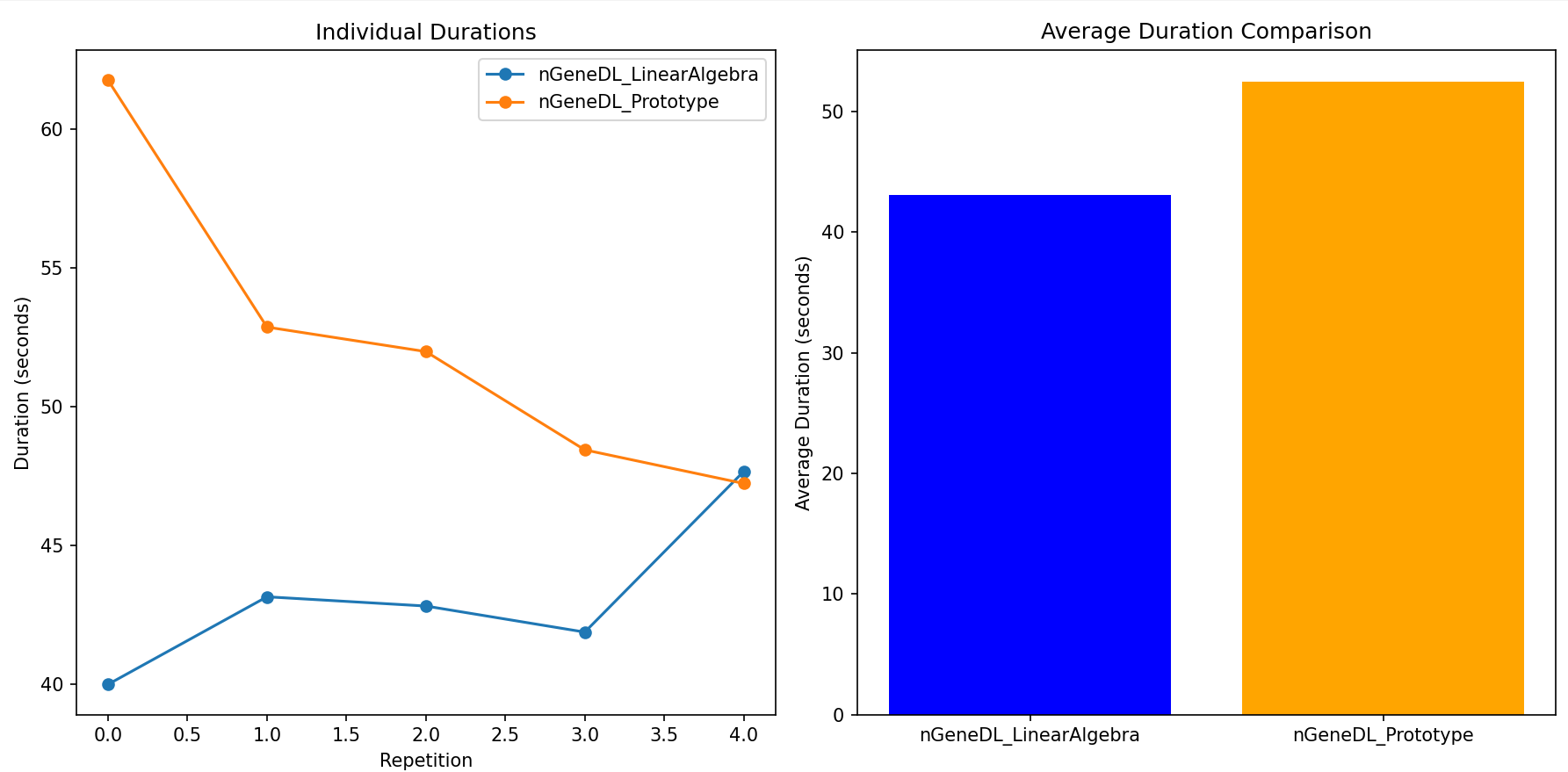
This result strongly indicates that nGeneDL_LinearAlgebra is more efficient overall, particularly in scenarios that require careful management of training duration and resource allocation.

Training Termination in the nGeneDL Class

(A) Efficient Model Training such as Early Stopping and Learning Rate Dynamics

In the extensive world of neural networks, deciding when to cease the training of a model is a critical consideration. Continuous training can lead to overfitting, where the model becomes excessively tailored to the training dataset, diminishing its generalization capability. Early stopping emerges as a pivotal solution to address this, intricately intertwining with model selection. This form of regularization avoids overfitting by halting training once a particular criterion is met, typically when performance on a validation dataset begins to degrade. The process involves periodically evaluating the model's performance on a validation set. If the validation metric stops improving or starts worsening, training continues for a predefined number of epochs, known as "patience." If no improvement occurs during this period, training is halted. Early stopping helps identify the iteration where the model offers the optimal balance between bias and variance, ensuring the selected model is neither underfitting nor overfitting.

Practitioners often start by testing a range of learning rates, typically on a logarithmic scale, and monitor the model’s convergence and validation performance for each rate. A dynamic approach, where the learning rate decreases over time, is often employed. Popular strategies include step decay, where the rate drops at specific epochs, and exponential decay, where it diminishes at a constant factor. Combining a higher initial learning rate with early stopping mechanisms can exploit the rapid convergence of a high rate while curtailing potential divergence. Analyzing the training loss curve is crucial; a smooth, descending curve indicates an appropriate learning rate, while oscillations or plateaus suggest adjustments are needed. Determining the optimal learning rate requires experimentation, intuition, and patience, ensuring the chosen rate aligns with the model’s architecture and the problem’s intricacies.

(B) How Training Decides When to Stop

The training process in the nGeneDL class is designed to be efficient and robust, utilizing techniques such as early stopping and learning rate adjustment. These methods help determine the optimal point to terminate training to prevent overfitting and ensure convergence.

B-1) Early Stopping: Early stopping is used to prevent the model from overfitting the training data by terminating training when the model's performance on a validation set stops improving. During each epoch, the model's loss is computed. If the current loss is better than the best loss observed so far (minus a small threshold min_delta), it is considered an improvement:

• The best loss is updated.
• The patience counter is reset.

if early_stopping:
     if loss < best_loss - min_delta:
        best_loss = loss
        patience_counter = 0
        lr_patience_counter = 0
     else:
        patience_counter += 1
        lr_patience_counter += 1
        if patience_counter >= patience:
           print(f"-> Early stopping at epoch {epoch + 1}")
           break

B-2) Learning Rate Adjustment: Adjusting the learning rate during training helps the model converge more effectively. If the learning rate is too high, the model might overshoot the optimal solution. If it is too low, the training process may become very slow. If the loss does not improve for a specified number of epochs (lr_patience), the learning rate is reduced by a factor (lr_factor):

• This reduction allows the model to make finer adjustments to weights, which is crucial as it approaches the optimal solution.
• The learning rate counter is reset after the adjustment.

if lr_patience_counter >= lr_patience:
     self.learning_rate *= lr_factor
     print(f"-> Reducing learning rate to {self.learning_rate} at epoch {epoch + 1}")
     lr_patience_counter = 0

B-3) Combined Use of Early Stopping and Learning Rate Adjustment: Combining early stopping and learning rate adjustment provides a balanced approach to training:

• Early Stopping: Ensures that training is terminated when improvements are minimal, preventing overfitting and saving computational resources.
• Learning Rate Adjustment: Allows for adaptive learning where the learning rate is decreased when the model's performance plateaus, facilitating finer weight updates and better convergence.

B-4) Threshold-based Early Stopping: The threshold-based early stopping mode in the nGeneDL class is a more aggressive training strategy designed for specific scenarios that may require extended training:

• Disables Early Stopping: Ensures that the model is given ample opportunity to converge, particularly useful for complex tasks or limited training data.
• Adjusts Learning Rate Patience and Factor: Provides more epochs before adjusting the learning rate and uses a more conservative reduction factor, allowing the model to explore the loss landscape more thoroughly.

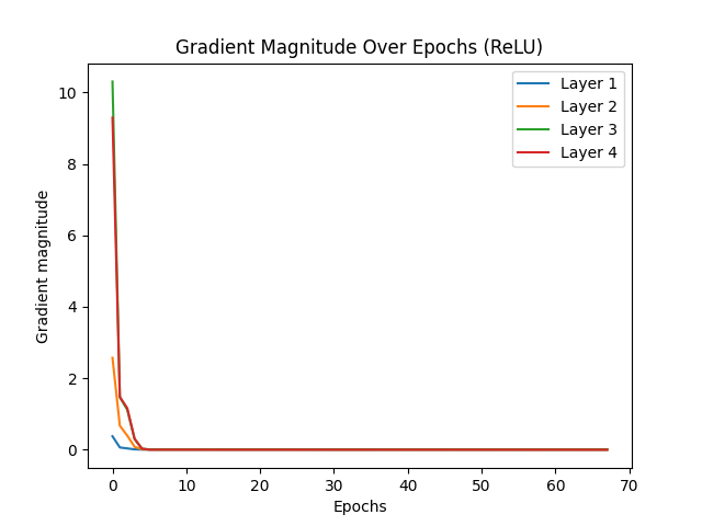
Vanishing Gradient Problem

The vanishing gradient problem is a significant challenge in training deep neural networks, particularly those with many layers. This issue arises during the backpropagation process, which updates the weights of a neural network by calculating the gradient of the loss function. When the gradients become exceedingly small, they essentially "vanish" as they propagate back through each layer, leading to very small updates for the earlier layers. This makes it difficult for the network to learn effectively, especially for deeper layers.

Backpropagation, a key algorithm for training neural networks, requires that the activation functions used by neurons be differentiable. Threshold activation functions, which output binary values, are not differentiable and therefore unsuitable for backpropagation. To overcome this, continuous activation functions such as logistic (sigmoid) and hyperbolic tangent (tanh) were introduced. However, these functions can still cause the vanishing gradient problem because their derivatives can become very small, especially when the inputs are far from zero. This results in gradients that diminish exponentially as they propagate through the network, making it difficult for the network to learn long-range dependencies.

(A) Mitigating the Vanishing Gradient Problem

The vanishing gradient problem began to be effectively addressed in the early 2000s and 2010s through several key developments:

• Long Short-Term Memory (LSTM): In 1997, Sepp Hochreiter and Jürgen Schmidhuber introduced the Long Short-Term Memory (LSTM) architecture, a type of recurrent neural network designed to mitigate the vanishing gradient problem in sequence learning tasks. LSTMs use gating mechanisms to maintain gradients during backpropagation, allowing them to capture long-term dependencies.
• ReLU/SoftPlus Activation Function: In 2011, the introduction of the Rectified Linear Unit (ReLU) activation function provided a simpler and more effective way to combat the vanishing gradient problem. ReLUs, unlike traditional sigmoid or tanh functions, do not saturate in the positive domain, helping to maintain larger gradients during training. However, ReLU has its limitations: it can "die" for negative inputs, leading to inactive neurons. To combat the issue of "dying" neurons in ReLU, variants like Leaky ReLU were developed. Leaky ReLU allows a small, non-zero gradient for negative inputs, ensuring that neurons continue to learn even when they receive negative signals. SoftPlus is another activation function that can be considered to address the issues with ReLU. The SoftPlus function is defined as:
  

  SoftPlus(x) = ln(1 + e^x)

  SoftPlus is a smooth approximation to ReLU and is always differentiable. Unlike ReLU, which has a sharp transition at zero, SoftPlus transitions smoothly, which can help in maintaining a stable gradient flow. For positive inputs, SoftPlus behaves similarly to ReLU, but for negative inputs, it does not completely shut down the gradients; instead, it allows small positive values, ensuring that neurons remain active and continue learning.
• Better Weight Initialization: Techniques for better weight initialization, such as Xavier (Glorot) initialization introduced by Xavier Glorot and Yoshua Bengio in 2010, helped mitigate the vanishing gradient problem by scaling weights to maintain consistent variance of activations throughout the network layers. Glorot initialization aims to maintain the variance of activations and gradients throughout the network. By initializing the weights in a way that keeps the variance of the outputs of each layer roughly equal, it ensures that the gradients neither vanish nor explode as they are propagated backward through the network. This method involves sampling the weights from a uniform distribution defined by the number of neurons in the input and output layers of each connection. Specifically, the weights are initialized using the formula:
  

  w ∼ U   [ - √(6 / (n_j + n_j+1)), √(6 / (n_j + n_j+1)) ]

  where n_j is the number of neurons in the current layer and n_j+1 is the number of neurons in the next layer. By using this initialization method, the variance of the activations and gradients is kept relatively constant throughout the network. This prevents the gradients from vanishing or exploding, which can occur if the weights are too small or too large, respectively.
• Batch Normalization: Introduced by Sergey Ioffe and Christian Szegedy in 2015, batch normalization normalizes the inputs of each layer, stabilizing the learning process and allowing for higher learning rates. This technique also helps address the vanishing gradient problem by maintaining healthy gradient magnitudes throughout training.

These developments collectively contributed to overcoming the vanishing gradient problem, enabling the successful training of much deeper neural networks and propelling the advancement of deep learning.

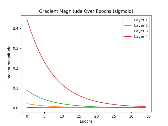
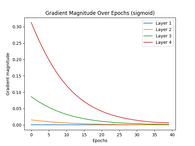
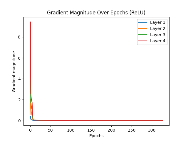
The vanishing gradient problem is a significant challenge in deep learning, particularly affecting activation functions like Sigmoid, which tend to cause gradients to diminish rapidly, halting effective learning. ReLU activation, by contrast, is less prone to vanishing gradients due to its nature, where gradients do not diminish to zero in positive activation regions. Glorot initialization, or Xavier initialization, aims to improve gradient flow by maintaining effective gradient magnitudes throughout the network. This initialization technique ensures that gradients neither vanish nor explode, leading to more efficient learning.

When comparing the test results for Sigmoid and ReLU activations with and without Glorot initialization, several observations stand out. Sigmoid activation without Glorot initialization converged quickly, stopping early at epoch 34 due to vanishing gradients. With Glorot initialization, Sigmoid showed slight improvement, stopping at epoch 39, indicating some mitigation of the vanishing gradient issue but still demonstrating its inherent limitations. On the other hand, ReLU activation without Glorot initialization required many epochs to converge, with early stopping at epoch 326. This slower convergence suggests that while gradients remained functional, they were not optimized, resulting in less efficient learning. However, with Glorot initialization, ReLU converged much faster, stopping at epoch 67. This faster convergence for ReLU with Glorot is a sign of efficient learning, as the network effectively reached an optimal solution more quickly.

In conclusion, the desired scenario for mitigating vanishing gradients is evident with ReLU activation combined with Glorot initialization. For ReLU, earlier convergence with Glorot initialization indicates efficient learning, as the network stops early due to reaching an optimal solution quickly. In contrast, Sigmoid activation, even with Glorot initialization, tends to stop early due to vanishing gradients, reflecting its inherent limitations. Thus, ReLU with Glorot initialization is the preferred combination for addressing the vanishing gradient problem, leading to more efficient and effective learning in deep networks.

Vanishing gradient test with sigmoid (without Glorot):

Reducing learning rate to 0.05 at epoch 29

Early stopping at epoch 34

Vanishing gradient test with sigmoid (with Glorot):

Reducing learning rate to 0.05 at epoch 34

Early stopping at epoch 39

Vanishing gradient test with ReLU (without Glorot):

Reducing learning rate to 0.05 at epoch 5

Reducing learning rate to 0.025 at epoch 315

Reducing learning rate to 0.0125 at epoch 321

Early stopping at epoch 326

Vanishing gradient test with ReLU (with Glorot):

Reducing learning rate to 0.05 at epoch 56

Reducing learning rate to 0.025 at epoch 62

Early stopping at epoch 67

Loss Function and Optimization Technique

Optimizing Machine Learning Models: MSE, Cross-Entropy Loss, and SGD

Mean Squared Error (MSE) and Cross-Entropy Loss are two widely used loss functions, each suited to different types of machine learning tasks. MSE is primarily used for regression tasks, measuring the average of the squared differences between the predicted and actual values. This makes it advantageous for continuous target variables due to its simplicity and smooth gradient, which benefits gradient-based optimization methods. However, MSE is highly sensitive to outliers because it penalizes larger errors more heavily, and its magnitude depends on the scale of the target variable, which can be problematic for variables with a wide range.

In contrast, Cross-Entropy Loss, also known as Logarithmic Loss, is typically used for classification tasks. It measures the difference between the true and predicted probability distributions. For binary classification, it is defined as the negative average of the sum of the true label times the log of the predicted probability and one minus the true label times the log of one minus the predicted probability. For multi-class classification, it extends to the negative average across all classes. Cross-Entropy Loss provides a probabilistic interpretation of predictions and heavily penalizes confidently incorrect predictions, making it effective for classification problems. It can handle imbalanced datasets well when combined with techniques like class weighting. However, its logarithmic nature can cause numerical instability if predictions are very close to 0 or 1, though this can be mitigated with label smoothing. Also, extremely confident predictions can lead to small gradients, potentially slowing down learning.

Stochastic Gradient Descent (SGD) and its variants are optimization techniques used to update model weights efficiently. Unlike batch gradient descent, which uses the entire dataset, SGD updates weights using a single data point or a small batch at each iteration. This leads to faster convergence, the ability to escape local minima, and introduces update variance. To address the limitations of SGD, several variants have been developed. Momentum accumulates velocity from previous gradients to smooth updates, Adagrad adjusts learning rates based on historical gradient values, and Adam combines elements of both Momentum and Adagrad, offering adaptive learning rates and smoother weight updates. These enhancements make SGD more robust and efficient.

SGD and its variants are particularly useful in scenarios involving large datasets, where computing the gradient over the entire dataset is computationally expensive. Using a single sample or small batch allows for faster updates. In online learning scenarios, where data arrives continuously or is frequently updated, SGD can continuously update the model without retraining on the entire dataset. For non-convex optimization, common in deep learning models, the stochastic nature of SGD helps escape local minima, finding better solutions. Additionally, when the dataset is too large to fit into memory, mini-batch SGD can be used as it requires only a small portion of the data to be loaded at a time.

Implementing MSE, Cross-Entropy Loss, and SGD in nGeneDL Code

In machine learning, selecting the appropriate loss function and optimization technique is crucial for effective model training. Two commonly used loss functions are Mean Squared Error (MSE) and Cross-Entropy Loss, each tailored to different types of tasks. Additionally, Stochastic Gradient Descent (SGD) and its variants offer flexible and efficient ways to optimize model weights. Below, we explore these concepts by quoting specific parts of the provided code, along with their corresponding mathematical equations.

(A) Mean Squared Error (MSE)

Mean Squared Error (MSE) is predominantly used in regression tasks where the goal is to predict continuous target variables. MSE measures the average of the squared differences between the predicted values and the actual values, which helps the model learn by minimizing these differences.

Equation:

MSE = (1/m) * Σ (yi - y_hati)2

In the provided code, MSE is implemented as follows:

if self.task == 'regression':
    loss = np.mean((self.a[-1] - y) ** 2)  # Mean Squared Error

Here, self.a[-1] represents the model's predictions, and y is the actual target values. The MSE loss function calculates the mean of the squared differences between these two, penalizing larger errors more heavily. This approach is beneficial for tasks requiring continuous output, as it ensures that the model learns to minimize large deviations from the target values.

(B) Cross-Entropy Loss

Cross-Entropy Loss, also known as Logarithmic Loss, is widely used in classification tasks. It measures the difference between the true label distribution and the predicted probability distribution. Cross-Entropy is particularly effective for classification because it penalizes incorrect predictions made with high confidence.

Equation (Binary Classification):

Cross-Entropy = - (1/m) * Σ [yi * log(y_hati) + (1 - yi) * log(1 - y_hati)]

Equation (Multi-Class Classification):

Cross-Entropy = - (1/m) * Σ Σ [yi,c * log(y_hati,c)]

Implementation of Cross-Entropy Loss

The relevant parts of the code for calculating Cross-Entropy Loss are:

if self.task == 'classification':
    dz = self.a[-1] - y  # Cross-Entropy Loss derivative

and

if self.task == 'classification':
    batch_loss = -np.mean(y_batch * np.log(self.a[-1] + 1e-15))  # Cross-Entropy Loss

Breakdown of the Code

Cross-Entropy Loss Derivative:

dz = self.a[-1] - y  # Cross-Entropy Loss derivative

self.a[-1]: Represents the predicted probabilities (y_hat_i for binary classification or y_hat_i,c for multi-class classification).

y: Represents the true labels, either as binary values (0 or 1) or one-hot encoded vectors for multi-class classification.

dz = self.a[-1] - y: This line calculates the derivative of the Cross-Entropy Loss with respect to the model's output (the predicted probabilities). It reflects how much the predicted probability deviates from the true label.

This derivative is crucial for updating the weights during backpropagation, as it guides the gradient descent process to minimize the loss.

Cross-Entropy Loss Calculation:

if self.task == 'classification':
    batch_loss = -np.mean(y_batch * np.log(self.a[-1] + 1e-15))  # Cross-Entropy Loss

Mathematical Translation:

Cross-Entropy = - (1/m) * Σ Σ [y_i,c * log(y_hat_i,c)]

Code Explanation:

np.mean(): Averages the loss over all samples in the batch. y_batch * np.log(self.a[-1] + 1e-15): This term calculates the log loss for each class and multiplies it by the true label (1 for the correct class, 0 for others). The small value 1e-15 is added to prevent taking the log of zero, which would result in a mathematical error.

Missing Components

The code effectively calculates Cross-Entropy Loss for multi-class classification. However, it does not explicitly handle the second term in the Cross-Entropy formula, which is necessary for binary classification:
- (1 - y_i) * log(1 - y_hat_i)
The current implementation focuses primarily on the term that addresses true positive cases:
y_i * log(y_hat_i)
For multi-class classification, the computation is handled correctly. However, the complementary part (1 - yi), which is relevant for binary classification scenarios, is not explicitly included. Consequently, while the code is appropriate for multi-class tasks, it may not fully account for cases where the model incorrectly predicts a high probability for the negative class in binary classification.

(C) Stochastic Gradient Descent (SGD) and Variants

Stochastic Gradient Descent (SGD) is an optimization technique that updates model weights incrementally using individual data points or small batches, rather than the entire dataset. This approach is computationally efficient and can help the model converge faster while escaping local minima.

Equation (SGD):

θt+1 = θt - η * ∇θ J(θ)

Equation (Momentum):

vt = β1 * vt-1 + η * ∇θ J(θ)
θt+1 = θt - vt

Equation (Adagrad):

Gt = Gt-1 + ∇θ J(θ) ⊙ ∇θ J(θ)
θt+1 = θt - (η / sqrt(Gt + ϵ)) * ∇θ J(θ)

Equation (Adam):

mt = β1 * mt-1 + (1 - β1) * ∇θ J(θ)
vt = β2 * vt-1 + (1 - β2) * (∇θ J(θ))2
m_hatt = mt / (1 - β1t)
v_hatt = vt / (1 - β2t)
θt+1 = θt - (η * m_hatt / (sqrt(v_hatt) + ϵ))

In the code, SGD and its variants are implemented in the backward method:

if self.optimizer == 'SGD':
    self.weights[i] -= self.learning_rate * dw  # Standard SGD update
elif self.optimizer == 'Momentum':
    self.velocity[i] = self.beta1 * self.velocity[i] + self.learning_rate * dw
    self.weights[i] -= self.velocity[i]  # Momentum update
elif self.optimizer == 'Adagrad':
    self.cache[i] += dw ** 2
    self.weights[i] -= self.learning_rate * dw / (np.sqrt(self.cache[i]) + self.epsilon)  # Adagrad update
elif self.optimizer == 'Adam':
    self.t += 1
    self.m[i] = self.beta1 * self.m[i] + (1 - the beta1) * dw
    self.v[i] = self.beta2 * self.v[i] + (1 - the beta2) * (dw ** 2)
    m_hat = self.m[i] / (1 - the beta1 ** self.t)
    v_hat = self.v[i] / (1 - the beta2 ** self.t)
    self.weights[i] -= self.learning_rate * m_hat / (np.sqrt(v_hat) + self.epsilon)  # Adam update

SGD: The standard SGD update adjusts the weights using the gradient (dw) scaled by the learning rate. This method is straightforward and allows for quick updates after each batch.

Momentum: This variant accumulates a velocity term (self.velocity[i]) that smooths the weight updates by considering past gradients, helping to accelerate the convergence.

Adagrad: Adagrad adjusts the learning rate based on the accumulated squared gradients (self.cache[i]). This adaptation helps the model handle sparse data or features by reducing the learning rate for frequently updated weights.

Adam: The Adam optimizer combines the benefits of Momentum and Adagrad by maintaining moving averages of both the gradients (self.m[i]) and the squared gradients (self.v[i]). Adam is particularly effective for deep learning models, offering adaptive learning rates and stability during training.

[Regression] In comparison to the control model (nGeneDL_LinearAlgebra using MSE), the nGeneDL_LinearAlgebra_SGD variants generally perform better with a batch size of 16 than with a batch size of 32, regardless of whether the learning rate is 0.01 or 0.1.

• SGD and its variants (Momentum, Adagrad, Adam) show faster convergence and reduced training times when the batch size is smaller (16), especially noticeable with SGD-Adam, which consistently achieves the quickest training times across different learning rates.
• For larger batch sizes (32), the performance of SGD variants tends to decrease slightly, leading to longer training times and less stable loss values compared to the smaller batch size.

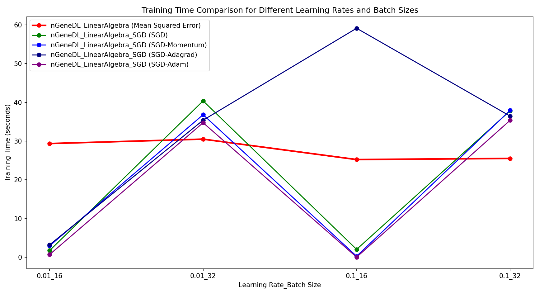
Overall, nGeneDL_LinearAlgebra_SGD demonstrates more efficient training with a batch size of 16, making it preferable for quicker convergence and stability in regression tasks.

[Classification] The results show that for classification tasks, standard SGD of nGeneDL_LinearAlgebra_SGD consistently outperforms both the control model (nGeneDL_LinearAlgebra using Cross-Entropy Loss) and the other SGD variants in all combinations of learning rates and batch sizes.

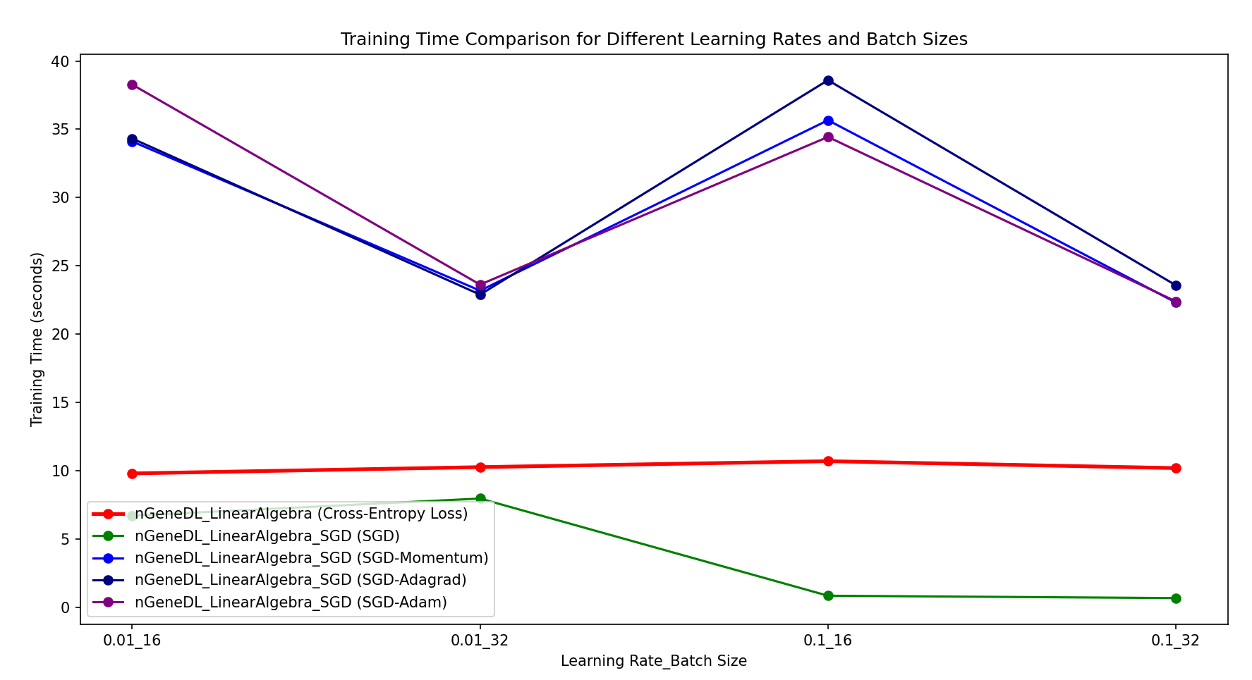
Specifically, standard SGD achieves faster training times and better efficiency compared to both the control model and the other variants (SGD-Momentum, SGD-Adagrad, SGD-Adam), regardless of the learning rate or batch size used.

Convolutional Neural Networks (CNNs)

How Convolutional Neural Networks Work

Convolutional Neural Networks (CNNs) are a class of deep neural networks specifically designed to automatically and adaptively learn spatial hierarchies of features from structured grid data, such as images. These networks are highly effective for image recognition and classification tasks, including applications like handwritten digit recognition. The core components of CNNs include convolutional layers, pooling layers, and fully connected layers, each playing a critical role in the network's functionality.

The convolutional layer is the fundamental building block of a CNN. It consists of a set of learnable filters (or kernels) that slide over the input image, performing convolution operations. These filters detect various features, such as edges, textures, and patterns, by computing the dot product between the filter and local regions of the input. As a result, the convolutional layer generates feature maps that highlight the presence of these features across the image. This process allows the network to learn spatial hierarchies of features, starting from low-level features in the initial layers to high-level, abstract features in deeper layers.

Pooling layers, often inserted between convolutional layers, reduce the spatial dimensions of the feature maps while retaining the most important information. The most common pooling operation is max pooling, which selects the maximum value from each patch of the feature map. Pooling layers help to downsample the data, reducing the computational load and the number of parameters in the network. They also contribute to the invariance of the network to small translations and distortions in the input image, enhancing its robustness.

Finally, fully connected layers, typically located at the end of the CNN, perform high-level reasoning and classification tasks. These layers take the flattened output from the last pooling or convolutional layer and process it through a series of neurons, each connected to every neuron in the previous layer. The fully connected layers integrate the spatially distributed features learned by the convolutional layers and produce the final output, such as class scores in classification tasks.

The combination of convolutional layers, pooling layers, and fully connected layers enables CNNs to effectively learn and recognize complex patterns in images, making them a powerful tool in the field of computer vision.

(A) Weight Sharing and Feature Detection

In a Convolutional Neural Network (CNN), each neuron functions as a visual feature detector by inspecting a small portion of the input image, known as its receptive field. Neurons in the first hidden layer receive specific pixel values as input and produce a high activation if a particular pattern or local visual feature is present within their receptive field.

The function implemented by a neuron is defined by the weights it uses—these weights are represented by the convolutional filter or kernel. When two neurons share the same set of weights but have different receptive fields (i.e., each neuron examines different areas of the input image), they both act as detectors for the same feature but in different locations. This property of sharing the same weights across different neurons is known as weight sharing.

Weight sharing is a fundamental characteristic of CNNs that allows for translation-invariant feature detection. This means that the network can detect the same feature, such as an edge or texture, regardless of where it appears in the image. Because the same filter is applied across the entire image, the network can recognize the feature in any position, making it robust to translations in the input.

(B) Stride Length and Overlapping Receptive Fields

The receptive fields of neurons can overlap, and the amount of overlap is controlled by a hyperparameter called the stride length. For example, if the stride length is one, the receptive field of the neuron is translated by one pixel at each step. Increasing the stride length reduces the overlap between receptive fields.

    Input image (5x5):
    [[1,  2,  3,  4,  5],
    [6,  7,  8,  9,  10],
    [11, 12, 13, 14, 15],
    [16, 17, 18, 19, 20],
    [21, 22, 23, 24, 25]]

    Filter (3x3):
    [[1, 2, 3],
    [4, 5, 6],
    [7, 8, 9]]

    Filter application (stride 1):
    [[1,  2,  3],
    [6,  7,  8],
    [11, 12, 13]]

    [[2,  3,  4],
    [7,  8,  9],
    [12, 13, 14]]

    ... and so on, with overlapping areas
  

    Input image (5x5):
    [[1,  2,  3,  4,  5],
    [6,  7,  8,  9,  10],
    [11, 12, 13, 14, 15],
    [16, 17, 18, 19, 20],
    [21, 22, 23, 24, 25]]

    Filter (3x3):
    [[1, 2, 3],
    [4, 5, 6],
    [7, 8, 9]]

    Filter application (stride 2):
    [[1,  2,  3],
    [6,  7,  8],
    [11, 12, 13]]

    [[3,  4,  5],
    [8,  9,  10],
    [13, 14, 15]]

    ... and so on, with less overlap
  

(C) Convolution Operation

In computer vision, the matrix of weights applied to an input is known as the kernel (or convolution mask). The operation of sequentially passing a kernel across an image and within each local region, weighting each input and adding the result to its local neighbors, is known as a convolution.

Convolving a kernel across an image is equivalent to passing a local visual feature detector across the image and recording all the locations in the image where the visual feature was present. The output from this process is a map of all the locations in the image where the relevant visual feature occurred. For this reason, the output of a convolution process is sometimes known as a feature map.

    1  2  3  4  5
    6  7  8  9  10
    11 12 13 14 15
    16 17 18 19 20
    21 22 23 24 25
  

    1  0 -1
    1  0 -1
    1  0 -1
  

    1  2  3
    6  7  8
    11 12 13
  

    1  0 -1
    1  0 -1
    1  0 -1
  

    1*1 + 2*0 + 3*(-1) + 6*1 + 7*0 + 8*(-1) + 11*1 + 12*0 + 13*(-1)
    = 1 + 0 - 3 + 6 + 0 - 8 + 11 + 0 - 13
    = -6
  

    -6  -6  -6  -6
    -6  -6  -6  -6
    -6  -6  -6  -6
    -6  -6  -6  -6
  

Relevant Code:

def conv2d(self, X, filter_size, stride):
    ...
    for i in range(0, input_height - filter_height + 1, stride):
        for j in range(0, input_width - filter_width + 1, stride):
           region = X[i:i + filter_height, j:j + filter_width]
           output[i // stride, j // stride] = np.sum(region)

(A) Weight Sharing and Feature Detection

• Weight Sharing: In your conv2d method, the same filter is applied to different regions of the input image as the nested loops iterate over it. This means the same weights are used across the image, ensuring that the feature is detected across different parts of the image.
• Feature Detection: The line output[i // stride, j // stride] = np.sum(region) computes the activation for each receptive field by summing up the values within the region, mimicking the detection of a specific feature represented by the filter.

(B) Stride Length and Overlapping Receptive Fields

• Stride Length: The stride parameter in the loops controls how many pixels the filter moves after each application. A smaller stride results in more overlap between consecutive receptive fields, whereas a larger stride reduces this overlap. In your code, the stride is set by the self.stride attribute when calling conv2d.

(C) Convolution Operation

• Convolution Operation: The conv2d function implements the convolution operation by taking a 2D input X, and applying a filter of size filter_size across it. The nested loops iterate over the image, selecting sub-regions (region) of the image, and computing the sum of the element-wise multiplication, which is stored in the output matrix.

(D) Activation Functions

The convolution operation in Convolutional Neural Networks (CNNs) does not inherently include a nonlinear activation function; it primarily involves a weighted summation of the inputs to identify basic patterns in the data, such as edges and textures. To capture more complex patterns, it is standard to apply a nonlinearity operation to the feature maps generated by convolutional layers. This is often accomplished using the Rectified Linear Unit (ReLU) activation function, defined as: rectifier(z) = max(0, z). The ReLU function introduces nonlinearity by transforming each position in the feature map, setting all negative values to zero while retaining positive values. This transformation allows the network to learn intricate patterns and relationships that linear operations alone cannot capture.

After convolution and ReLU activation, the next critical step is dimensionality reduction, achieved through pooling layers. Pooling layers, such as max pooling, are employed to condense the features extracted by the convolutional layers, reducing the spatial dimensions of the data. This process retains only the most important aspects of the feature maps, leading to a more manageable and robust representation of the input. Pooling helps the network become less sensitive to variations such as translations or noise, thereby enhancing its ability to generalize from the input data.

The typical sequence of operations in CNNs, namely Convolution → ReLU Activation → Max Pooling, works synergistically to extract meaningful features, introduce nonlinearity, and efficiently down-sample the data, creating a powerful framework for tasks like image recognition and classification.

def relu(self, X):
    return np.maximum(0, X)

• ReLU Activation: The relu function is applied to the output of the convolutional layer to introduce non-linearity. This function replaces all negative values in the feature map with zero, which allows the network to learn complex patterns by stacking multiple layers.

(E) Pooling

Pooling operations in Convolutional Neural Networks (CNNs) are crucial techniques used to reduce the spatial dimensions of input feature maps while preserving important information. Like convolution operations, pooling involves repeatedly applying a function across an input space, but its primary goal is to down-sample the feature maps, decreasing computational complexity and mitigating overfitting by making the representation smaller and more manageable.

There are two main types of pooling used in CNNs: max pooling and average pooling. Max pooling selects the maximum value from a defined region, or pooling window, effectively capturing the most prominent feature in that region. This makes max pooling particularly effective for retaining sharp, high-intensity features. In contrast, average pooling calculates the average value of the inputs within the pooling window, providing a more generalized representation of the features and smoothing out noise. Both techniques operate over a small region of the input feature map, known as the receptive field.

The size of the receptive field determines the region over which the pooling function operates, and the stride determines how far the pooling window moves after each operation. If the stride is greater than one, the pooling windows do not overlap, resulting in a more significant reduction in spatial dimensions. This non-overlapping nature ensures distinct regions are sampled, whereas overlapping windows may capture more detail but require more computational resources.

In CNNs, the typical sequence of operations involves applying convolutional filters to the input image to generate feature maps, followed by the application of non-linear activation functions like ReLU (Rectified Linear Unit) to introduce nonlinearity. This is then followed by pooling, which helps down-sample the feature maps. By reducing the height and width of these maps, pooling helps the network become invariant to small translations and distortions in the input image, significantly lowering the number of parameters and operations required. This makes the network more efficient, enabling faster training and inference, which is especially beneficial for large-scale and real-time applications.

    1  3  2  4
    5  6  1  2
    9  8  7  6
    4  3  2  1
  

    1  3
    5  6
  

    2  4
    1  2
  

    9  8
    4  3
  

    7  6
    2  1
  

    6  4
    9  7
  

    1  3
    5  6
  

    2  4
    1  2
  

    9  8
    4  3
  

    7  6
    2  1
  

    3.75  2.25
    6.00  4.00
  

def max_pooling(self, X, pool_divisions):
    input_height, input_width = X.shape
    pool_size = input_height // pool_divisions
    output = np.zeros((pool_divisions, pool_divisions))

    for i in range(pool_divisions):
       for j in range(pool_divisions):
          region = X[i * pool_size:(i + 1) * pool_size, j * pool_size:(j + 1) * pool_size]
          output[i, j] = np.max(region)

    return output

• Max Pooling: The max_pooling method performs max pooling by dividing the feature map into non-overlapping regions based on the pool_divisions parameter. For each region, it takes the maximum value, effectively down-sampling the feature map and retaining the most significant features.
• Reduction in Spatial Dimensions: By selecting the maximum value from each pooling region, this function reduces the spatial size of the feature map, which helps in reducing computational load and makes the network more robust.

(F) Multiple Convolutional Layers and Filters

A CNN can generalize beyond one feature by training multiple convolutional layers in parallel (or filters), with each filter learning a single kernel matrix (feature detection function). The outputs of multiple filters can be integrated in a variety of ways. One way is to combine the feature maps generated by separate filters into a single multifilter feature map. A subsequent convolutional layer then takes this multifilter feature map as input.

The nGeneCNN_MultipleFilters Class: The nGeneCNN_MultipleFilters class extends the functionality of the nGeneCNN_Prototype class to support multiple convolutional filters. This enhancement aligns with the concept of having multiple convolutional layers and filters in a CNN, which allows the network to generalize beyond detecting a single feature and instead detect multiple distinct features within the input data.

1. Initialization of Multiple Filters

def __init__(self, filter_size=(3, 3), stride=2, pool_divisions=-1, num_filters=3, percentage_combinations=100, debug_backpropagation=False):
    super().__init__(filter_size=filter_size, stride=stride, pool_divisions=pool_divisions, debug_backpropagation=debug_backpropagation)
    self.num_filters = num_filters
    self.percentage_combinations = percentage_combinations
    self.filters = self.initialize_filters()

• The __init__ method initializes multiple filters for the convolutional layer. The number of filters is determined by the num_filters parameter.
• initialize_filters generates these filters randomly, which allows each filter to potentially learn a different feature during the training process.

2. Filter Initialization

def initialize_filters(self):
    total_combinations = 2 ** (self.filter_size[0] * self.filter_size[1])
    num_filters_to_generate = int((self.percentage_combinations / 100.0) * total_combinations)
    filters = np.random.randn(min(self.num_filters, num_filters_to_generate), self.filter_size[0], self.filter_size[1])
    return filters

• The initialize_filters method generates a set of filters based on the specified filter_size, num_filters, and percentage_combinations.
• This ensures that each filter is unique and can detect different features within the input data, allowing the network to capture a broader range of patterns.

3. Convolution with Multiple Filters

def conv2d(self, X, filter_size, stride):
    filter_height, filter_width = filter_size
    input_height, input_width = X.shape
    output_height = (input_height - filter_height) // stride + 1
    output_width = (input_width - filter_width) // stride + 1
    output = np.zeros((self.num_filters, output_height, output_width))

    for f in range(self.num_filters):
       for i in range(0, input_height - filter_height + 1, stride):
          for j in range(0, input_width - filter_width + 1, stride):
             region = X[i : i + filter_height, j : j + filter_width]
             output[f, i // stride, j // stride] = np.sum(region * self.filters[f])

    return output

• The conv2d method has been modified to perform convolution operations using multiple filters.
• For each filter, the method iterates over the input data and applies the filter to different regions of the input.
• The result is a set of feature maps, one for each filter, which are stored in a 3D output array (where each "slice" along the first dimension corresponds to the feature map from one filter).

4. Max Pooling Across Multiple Feature Maps

def max_pooling(self, X, pool_divisions):
    num_filters, input_height, input_width = X.shape
    pool_size = input_height // pool_divisions
    output = np.zeros((num_filters, pool_divisions, pool_divisions))

    for f in range(num_filters):
       for i in range(pool_divisions):
          for j in range(pool_divisions):
             region = X[f, i * pool_size : (i + 1) * pool_size, j * pool_size : (j + 1) * pool_size]
             output[f, i, j] = np.max(region)

    return output

• The max_pooling method applies max pooling independently to each feature map generated by the filters.
• This method processes each feature map separately, down-sampling it by taking the maximum value within each pooling region.
• This reduces the spatial dimensions of each feature map while retaining the most important information, thereby making the feature maps more manageable for further processing.

5. Visualization of Filters and Feature Maps

def visualize_filters(self):
    num_filters = len(self.filters)
    fig, axes = plt.subplots(1, num_filters, figsize=(15, 5))
    for i, ax in enumerate(axes):
       ax.imshow(self.filters[i], cmap='gray')
       ax.set_title(f'Filter {i+1}')
       ax.axis('off')
    plt.show()

def visualize_feature_maps(self, feature_maps, title="Feature Maps"):
    num_feature_maps = feature_maps.shape[0]
    fig, axes = plt.subplots(1, num_feature_maps, figsize=(15, 5))
    for i, ax in enumerate(axes):
       ax.imshow(feature_maps[i], cmap='gray')
       ax.set_title(f'Feature Map {i+1}')
       ax.axis('off')
    plt.suptitle(title)
    plt.show()

• visualize_filters allows for the visualization of each filter, making it possible to inspect what each filter has learned.
• visualize_feature_maps enables the visualization of the resulting feature maps after applying the filters and pooling, helping to understand which features are being detected by the network.

Example: Handwritten Digit Recognition

In the context of handwritten digit recognition, a CNN might receive an input image of a digit (e.g., 28x28 pixels). The first layer could apply several convolutional filters to detect edges and simple shapes. Subsequent layers would detect more complex features, such as curves and digit-like shapes, by combining the features detected in previous layers. Pooling layers would reduce the spatial dimensions, preserving the most important information. Finally, dense layers would integrate these features to classify the image as one of the ten possible digits (0-9).

By leveraging weight sharing, convolutional operations, activation functions, and pooling, CNNs efficiently and effectively recognize patterns in images, making them powerful tools for tasks like handwritten digit recognition.

Overview of Training Approaches

This analysis explores three primary training methods on the MNIST digit recognition task:

• No CNN, Cross Entropy Loss Optimization: Utilizes a fully connected neural network trained with Cross Entropy Loss, without any convolutional layers.
• No CNN, SGD Optimization: Similar to the first method but uses Stochastic Gradient Descent (SGD) and its variants as the optimization method.
• CNN with Single Filter, Comparison of Time & Accuracy: Introduces a single convolutional filter and compares performance across different optimizers, focusing on both training time and accuracy.

(A) No CNN with Cross Entropy Loss Optimization

In the train_and_test_mnist_no_cnn_nGeneDL_LinearAlgebra function, a fully connected neural network is trained on the MNIST dataset using Cross Entropy Loss as the loss function. This method does not utilize any convolutional layers, and the network relies solely on dense layers to learn the digit patterns.

=== [Digit Recognition] no CNN by Cross Entropy Loss Optimization ===
  Epoch 1/1000: Loss = 0.2454645
  Epoch 201/1000: Loss = 0.0386511
  Epoch 401/1000: Loss = 0.0301550
  Epoch 601/1000: Loss = 0.0268234
  Epoch 801/1000: Loss = 0.0242453
  => Test set accuracy: 0.9287

• Training: The network is trained over 1000 epochs, with threshold-based early stopping if the loss falls below a certain threshold.
• Performance: While this method achieves a test accuracy of approximately 92.87%, it takes significantly longer to converge, as indicated by the gradual decrease in loss over the epochs.

nn = nGeneDL_LinearAlgebra(input_nodes=784, output_nodes=10, hidden_nodes=[128, 64], learning_rate=0.1)
nn.fit(X_train.T, Y_train_one_hot, epochs=1000, threshold_based_early_stopping=True)
test_predictions = nn.predict(X_test.T)
accuracy = np.sum(test_predictions.flatten() == Y_test) / Y_test.size
print(f"=> Test set accuracy: {accuracy}")

• Epochs: 1000 (with early stopping).
• Final Loss: 0.0242453.
• Test Accuracy: 0.9287.

(B) No CNN with SGD Optimization

The train_and_test_mnist_no_cnn_nGeneDL_LinearAlgebra_SGD function also trains a fully connected network but uses various SGD-based optimizers, including Momentum, Adagrad, and Adam. This method improves both convergence speed and accuracy compared to Cross Entropy Loss optimization.

=== [Digit Recognition] no CNN by SGD Optimization with Single Filter ===
  Training with optimizer: SGD, learning rate: 0.01, batch size: 32
  Epoch 1/1000: Loss = 0.1041797
  -> Threshold-based early stopping at epoch 28 with loss 0.0041823 as loss < 0.005.
  ===> Test set accuracy: 0.9257
    
  Training with optimizer: Momentum, learning rate: 0.01, batch size: 32
  Epoch 1/1000: Loss = 0.0766008
  -> Threshold-based early stopping at epoch 14 with loss 0.0010442 as loss < 0.005.
  ===> Test set accuracy: 0.9556

  Training with optimizer: Adagrad, learning rate: 0.01, batch size: 32
  Epoch 1/1000: Loss = 0.0209173
  -> Threshold-based early stopping at epoch 4 with loss 0.0042766 as loss < 0.005.
  ===> Test set accuracy: 0.9350

  Training with optimizer: Adam, learning rate: 0.01, batch size: 32
  Epoch 1/1000: Loss = 0.0443852
  -> Threshold-based early stopping at epoch 3 with loss 0.0041846 as loss < 0.005.
  ===> Test set accuracy: 0.9444

• Training: The network is trained using different optimizers, which adjust the learning rate dynamically or incorporate momentum to accelerate convergence.
• Performance: With optimizers like Momentum and Adam, the network achieves higher accuracy (up to 95.56%) and converges much faster, often within a few epochs.

nn_sgd = nGeneDL_LinearAlgebra_SGD(input_nodes=784, output_nodes=10, hidden_nodes=[128, 64], learning_rate=0.01, optimizer='Adam')
nn_sgd.fit(X_train.T, Y_train_one_hot, epochs=1000, batch_size=32, early_stopping=False)
test_predictions = nn_sgd.predict(X_test.T)
accuracy = np.sum(test_predictions.flatten() == Y_test) / Y_test.size
print(f"===> Test set accuracy: {accuracy:.4f}")

• Best Optimizer: Momentum (Accuracy: 0.9556).
• Fastest Convergence: Adam (Converged within 2-4 epochs).
• Test Accuracy Range: 0.9257 to 0.9556.

(C) CNN with Single Filter: Time & Accuracy Comparison

The train_and_test_mnist_cnn_SGD_comparision_time_accuracy_without_prediction function introduces a CNN architecture with a single convolutional filter. The function compares the performance of the Cross Entropy Loss and various SGD optimizers in terms of both training time and accuracy.

=== [Digit Recognition] CNN by SGD Optimizations with Single Filter for Comparison: Time & Accuracy ===
  Original raw input dimensions: (28, 28)
  Feature map dimension after convolution: (26, 26)
  Possible non-overlapping pool divisions: [1, 2, 13]
  => Maximum non-overlapping pool divisions possible (excluding feature map dimension): 13

  Processing image for X_train_processed:..........
  Processing image for X_test_processed :..........
  => Number of Input nodes: 169

  === Training Time & Prediction Accuracy ===
  Epoch 1/1000: Loss = 0.5406638
  Epoch 201/1000: Loss = 0.0386366
  Epoch 401/1000: Loss = 0.0309034
  Epoch 601/1000: Loss = 0.0270548
  Epoch 801/1000: Loss = 0.0244385
  ===> nGeneDL_LinearAlgebra (Cross Entropy Loss) training time: 73.79 seconds
  ===> Test set accuracy for nGeneDL_LinearAlgebra (Cross Entropy Loss): 0.9304

  Epoch 1/1000: Loss = 0.0581560
  -> Threshold-based early stopping at epoch 2 with loss 0.0046510 as loss < 0.005.
  ===> nGeneDL_LinearAlgebra_SGD (SGD) training time: 0.22 seconds
  ===> Test set accuracy for nGeneDL_LinearAlgebra_SGD (SGD): 0.9018

  Epoch 1/1000: Loss = 0.0415230
  -> Threshold-based early stopping at epoch 7 with loss 0.0020228 as loss < 0.005.
  ===> nGeneDL_LinearAlgebra_SGD (Momentum) training time: 0.80 seconds
  ===> Test set accuracy for nGeneDL_LinearAlgebra_SGD (Momentum): 0.9642

  Epoch 1/1000: Loss = 0.0135918
  -> Threshold-based early stopping at epoch 4 with loss 0.0047833 as loss < 0.005.
  ===> nGeneDL_LinearAlgebra_SGD (Adagrad) training time: 0.54 seconds
  ===> Test set accuracy for nGeneDL_LinearAlgebra_SGD (Adagrad): 0.9524

  Epoch 1/1000: Loss = 0.0191139
  -> Threshold-based early stopping at epoch 2 with loss 0.0042699 as loss < 0.005.
  ===> nGeneDL_LinearAlgebra_SGD (Adam) training time: 0.28 seconds
  ===> Test set accuracy for nGeneDL_LinearAlgebra_SGD (Adam): 0.9103

• CNN Architecture: A single convolutional filter is applied, followed by max pooling. The processed data is then passed to a fully connected network.
• Training Efficiency: This method significantly reduces training time while maintaining high accuracy, especially when using optimizers like Momentum and Adam.

preprocessor = nGeneCNN_Prototype(filter_size=(3, 3), stride=1)
X_train_processed = preprocessor.preprocess(X_train)
X_test_processed = preprocessor.preprocess(X_test)

nn = nGeneDL_LinearAlgebra(input_nodes=X_train_processed.shape[1], output_nodes=10, hidden_nodes=[128, 128], learning_rate=0.01)
nn.fit(X_train_processed, Y_train_one_hot, epochs=1000, threshold_based_early_stopping=True)
test_predictions = nn.predict(X_test_processed)
accuracy = np.sum(test_predictions.flatten() == Y_test) / Y_test.size
print(f"===> Test set accuracy: {accuracy}\n")

• Cross Entropy Loss Training Time: 73.79 seconds.
• Best Optimizer: Momentum (Accuracy: 0.9642, Training Time: 0.80 seconds).
• Test Accuracy Range: 0.9018 to 0.9642.

(D) Analysis of Digit Recognition Using CNN with Multiple Filters

This analysis examines the application of Convolutional Neural Networks (CNNs) with three filters to the MNIST digit recognition task. The objective is to compare the performance of two frameworks: nGeneDL_LinearAlgebra using Cross Entropy Loss, and nGeneDL_LinearAlgebra_SGD using Stochastic Gradient Descent (SGD) and its variants (Momentum, Adagrad, and Adam). The focus is on evaluating each method in terms of both training efficiency and accuracy.

Multiple Filters and Feature Visualization: Prior to discussing the results, the model visualizes the initial random filters and their processing of the hand-digit images. This visualization is crucial for understanding how each filter detects different aspects of the digits, such as edges, textures, or shapes.

• Filter Visualization: The three filters begin with random weights, which evolve as the network undergoes training. Each filter is designed to focus on different features within the image, contributing to a more comprehensive understanding of the data.

• Feature Map Visualization: Following the convolution operation, the resulting feature maps highlight the areas of the image that each filter finds significant, providing insights into the learning process.

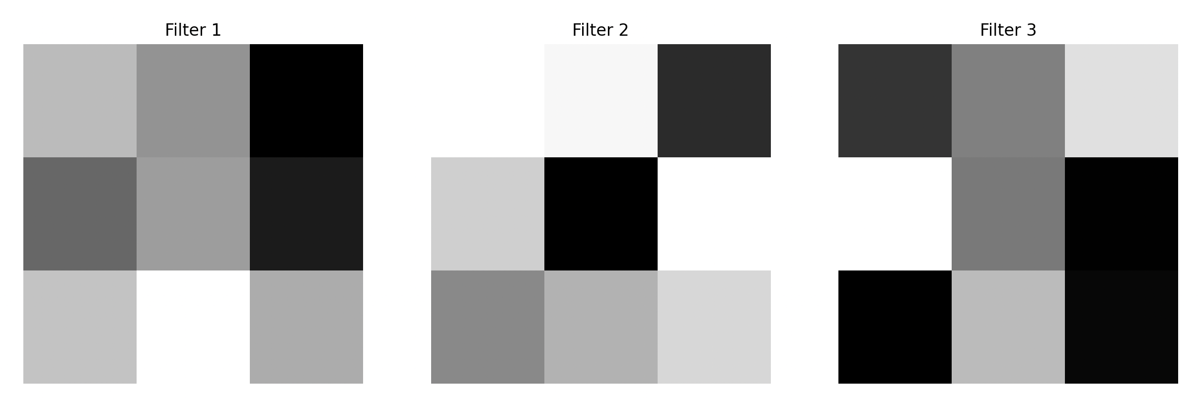
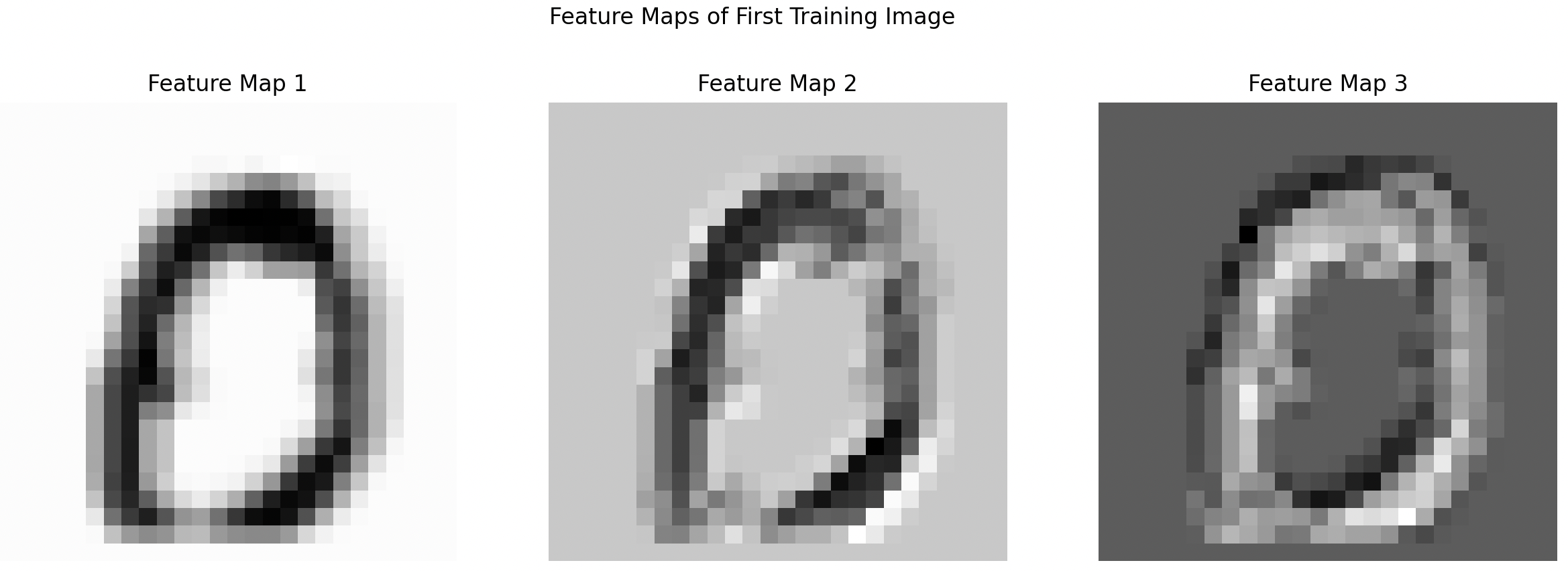
D-1) nGeneDL_LinearAlgebra with Cross Entropy Loss

The train_and_test_mnist_cnn_multiple_filters function tests the CNN with multiple filters using the nGeneDL_LinearAlgebra framework and Cross Entropy Loss. The model is trained for a full 1000 epochs, as the loss does not drop below 0.005 before reaching the later epochs.

• Training Duration: The network completes all 1000 epochs because the reduction in loss is gradual, requiring the entire training period to achieve the desired level.
• Test Accuracy: The model achieves a test set accuracy of 92.84%, demonstrating strong performance, albeit with longer training times.
• Loss Trajectory: The loss decreases steadily over time, indicating that the model is learning effectively, though at a slower pace compared to other optimizers.

Epoch 1/1000: Loss = 0.3411547
Epoch 201/1000: Loss = 0.0410656
Epoch 401/1000: Loss = 0.0298363
Epoch 601/1000: Loss = 0.0254221
Epoch 801/1000: Loss = 0.0229610
=> Test set accuracy: 0.9284

D-2) nGeneDL_LinearAlgebra_SGD with SGD or its variants

The train_and_test_mnist_cnn_SGD_multiple_filters function evaluates the CNN with multiple filters using the nGeneDL_LinearAlgebra_SGD framework with various SGD-based optimizers. The results demonstrate that these optimizers significantly reduce the training time by triggering threshold-based early stopping when the loss drops below 0.005.

a. SGD Optimizer

• Training Duration: The model stops at epoch 15, as the loss quickly falls below the threshold.
• Test Accuracy: The test accuracy reaches 93.63%, indicating a good balance between training speed and model performance.

Epoch 1/1000: Loss = 0.0986447
-> Threshold-based early stopping at epoch 15 with loss 0.0048741 as loss < 0.005.
===> Test set accuracy for nGeneDL_LinearAlgebra_SGD (SGD): 0.9363

b. Momentum Optimizer

• Training Duration: The fastest optimizer in this comparison, stopping at epoch 5 with a loss of 0.0035961.
• Test Accuracy: Momentum achieves the highest accuracy at 96.21%, demonstrating its effectiveness in quickly converging to an optimal solution.

Epoch 1/1000: Loss = 0.0264336
-> Threshold-based early stopping at epoch 5 with loss 0.0035961 as loss < 0.005.
===> Test set accuracy for nGeneDL_LinearAlgebra_SGD (Momentum): 0.9621

c. Adagrad Optimizer

• Training Duration: Similar to Momentum, Adagrad stops early at epoch 5, but with a slightly higher loss of 0.0040192.
• Test Accuracy: Adagrad achieves a strong test accuracy of 95.87%, making it another viable option for this task.

Epoch 1/1000: Loss = 0.0594092
-> Threshold-based early stopping at epoch 5 with loss 0.0040192 as loss < 0.005.
===> Test set accuracy for nGeneDL_LinearAlgebra_SGD (Adagrad): 0.9587

d. Adam Optimizer

• Training Duration: Adam converges the fastest, stopping at epoch 3 with a loss of 0.0022884.
• Test Accuracy: While not the highest, Adam still achieves a robust accuracy of 94.85%, highlighting its efficiency in minimizing loss quickly.

Epoch 1/1000: Loss = 0.0545857
-> Threshold-based early stopping at epoch 3 with loss 0.0022884 as loss < 0.005.
===> Test set accuracy for nGeneDL_LinearAlgebra_SGD (Adam): 0.9485

Conclusion

• Training Efficiency: nGeneDL_LinearAlgebra_SGD with SGD or its variants consistently finishes earlier than nGeneDL_LinearAlgebra with Cross Entropy Loss. Among the SGD variants, Momentum emerges as the best in terms of both speed and accuracy, followed closely by Adagrad and Adam.
• Test Accuracy: While all methods achieve strong test accuracy, Momentum stands out with the highest accuracy of 96.21%.
• Recommendation: For browser-based or time-sensitive applications, nGeneDL_LinearAlgebra_SGD with Momentum or Adam is recommended due to their quick convergence and high accuracy.

By leveraging multiple filters and the appropriate optimizer, the model efficiently processes digit images, leading to faster training times and better generalization on test data.

Reference (listed in order of greatest to least influence)

• Kelleher, J. D. (2019). Deep Learning. MIT Press. ISBN: 9780262537551.
• Starmer, J. (n.d.; 2022). StatQuest with Josh Starmer [YouTube channel] and The StatQuest Illustrated Guide To Machine Learning. StatQuest Publications. ISBN-13: 979-8986924007. Retrieved from https://www.youtube.com/watch?v=zxagGtF9MeU&list=PLblh5JKOoLUIxGDQs4LFFD--41Vzf-ME1

---

• Zhang, S. (n.d.). Simple MNIST NN from scratch (numpy, no TF/Keras) [Video and source code]. YouTube; Kaggle. Retrieved from https://www.youtube.com/watch?v=w8yWXqWQYmU&t=13s and https://www.kaggle.com/code/wwsalmon/simple-mnist-nn-from-scratch-numpy-no-tf-keras
• Knowings, L. D. (2024). Building neural networks from scratch with Python. Independently published.

---

• Géron, A. (2022). Hands-On Machine Learning with Scikit-Learn, Keras, and TensorFlow: Concepts, Tools, and Techniques to Build Intelligent Systems (3rd ed.). O'Reilly Media.
• Raschka, S., & Mirjalili, V. (2019). Python Machine Learning: Machine Learning and Deep Learning with Python, scikit-learn, and TensorFlow 2 (3rd ed.). Packt Publishing.
• Raschka, S., & Liu, Y. (2022). Machine Learning with PyTorch and Scikit-Learn: Develop machine learning and deep learning models with Python. Packt Publishing.
• NeuralNine. (n.d.). NeuralNine [YouTube channel]. Retrieved from https://www.youtube.com/@NeuralNine

Support Vector Machine (SVM)

A Classifier for Small Datasets, Supplementing Deep Learning

Introduction to the Fundamentals of SVM

Why It’s Called "Support Vector Machine": The name "Support Vector Machine" (SVM) reflects the key concept behind this powerful classification model. At the heart of SVM are "support vectors"—these are the critical data points that lie closest to the decision boundary, also known as the hyperplane. Imagine trying to draw a line (in two dimensions) or a plane (in three dimensions) that separates two groups of points. The support vectors are the points that are nearest to this line or plane. They essentially "support" or define the decision boundary, ensuring that it is positioned in a way that maximizes the distance (margin) between the classes. By focusing on just these key points, SVM efficiently determines the best boundary to distinguish between different classes, which is why it’s named after these pivotal elements.

How SVM Works: At its core, SVM is a classification technique that strives to separate data points into distinct groups with as wide a margin as possible. To achieve this, SVM may map the original data into a higher-dimensional space where it becomes easier to separate the classes. This mapping is accomplished through the use of kernel functions—mathematical tools that enable SVM to perform complex transformations without needing to explicitly compute the coordinates in the higher dimension. This process is crucial for handling cases where the data is not linearly separable in its original form.

For instance, if you have data points that are arranged in a circular pattern, it might be impossible to separate them with a straight line in two dimensions. However, by projecting these points into a higher dimension (for example, by adding a third dimension), SVM can find a hyperplane that separates them. The ability to find the optimal separating hyperplane, one that maximizes the margin between the nearest points of each class, is what makes SVM particularly effective for both linear and nonlinear classification problems. Whether you’re dealing with simple or complex datasets, SVM can adapt by selecting the appropriate kernel function, such as the polynomial kernel or the radial basis function (RBF) kernel.

Benefits of SVM: SVMs are celebrated for their precision and reliability, especially when working with complex datasets that are small to medium in size. They often deliver high performance "right out of the box," requiring minimal tweaking or optimization, which makes them a go-to choice for many machine learning tasks. One of the standout features of SVMs is their versatility—they aren’t just limited to classification tasks. SVMs can also be used for regression and outlier detection, making them highly adaptable to various problem domains. This flexibility is largely due to the kernel trick, which allows SVMs to effectively manage nonlinear data by transforming it into a space where it becomes linearly separable. This transformation, achieved without actually computing in the high-dimensional space, is both efficient and powerful.

Moreover, SVMs are less susceptible to overfitting, which is a common problem in machine learning where a model performs well on training data but poorly on unseen data. SVMs mitigate this risk by focusing on maximizing the margin between classes, which leads to a more generalized model. Additionally, they can handle outliers and tolerate some degree of misclassification (a concept known as soft margin), making them robust in real-world applications where perfect separation of classes is not always possible. Whether in image recognition, bioinformatics, or any other field where data may be complex and not perfectly separable, SVMs provide a reliable and effective solution.

The Kernel Trick: Both the Polynomial and RBF kernels utilize the Kernel Trick to calculate the relationships between data points as if they were in higher dimensions. This ingenious approach allows SVMs to classify complex datasets efficiently by computing dot products in these expanded feature spaces without the need for explicit, computationally expensive transformations. Through the application of kernel functions, SVMs can effectively handle linearly inseparable data, making them versatile tools for a wide range of machine learning tasks.

Understanding the Limits of 2D Decision Boundary Visualizations: When visualizing decision boundaries in 2D for high-dimensional datasets, it's important to recognize that these plots can sometimes be misleading. The key issue is that the decision boundaries learned by an SVM (or any other model) in a higher-dimensional space may not translate accurately when projected down to two dimensions.

from sklearn.datasets import make_classification
X_high_dim, y_high_dim = make_classification(n_samples=100, n_features=5, n_informative=5, n_redundant=0, n_clusters_per_class=1, random_state=42)

When training an SVM model on data in a 5-dimensional space (n_features=5), the classes may be perfectly separable using a specific kernel and parameter set, as the separability depends on relationships and structures across all five dimensions. However, when this 5D space is reduced to 2D using techniques like PCA (Principal Component Analysis), the complex multi-dimensional decision boundary is projected onto a two-dimensional plane, often distorting the original boundary. This projection can make the decision boundary appear less optimal or even incorrect in 2D, leading to potential misinterpretations. PCA aims to preserve as much variance as possible, but it cannot fully capture the intricate relationships and separability of the original high-dimensional space. Consequently, while a decision boundary in 2D might seem suboptimal or misleading, it could still be highly accurate in the full 5D space, highlighting the importance of understanding the limitations of 2D visualizations.

When evaluating a model's performance, it's essential to prioritize cross-validation accuracy over 2D decision boundary visualizations. Cross-validation provides a more accurate reflection of the model's true performance, as it considers the full-dimensional space of the data, rather than the simplified 2D projection. While decision boundary plots can offer a rough visual understanding of how the model separates data, they should be interpreted with caution, as they may not fully capture the complexity and effectiveness of the model in higher dimensions.

Comparing Deep Learning and SVM

Understanding Kernel Functions in SVMs

Kernel functions are essential tools that allow Support Vector Machines (SVMs) to handle complex data by mapping it into higher-dimensional spaces. The genius of kernel functions lies in their ability to compute relationships between data points in these higher dimensions without actually transforming the data into those dimensions. This clever approach, known as the "Kernel Trick," drastically reduces the computational burden, especially when dealing with large datasets or spaces that would otherwise be infinitely complex.

(A) Polynomial Kernel

The Polynomial Kernel is a powerful example of how SVMs can classify data by projecting it into a higher-dimensional space. By increasing the dimensions in which we consider the data, we can find a separating boundary (or hyperplane) that might not be evident in the original space.

The Polynomial Kernel is defined mathematically as (x ⋅ z + r)d, where:

• x and z are vectors representing data points in the dataset.
• r is a coefficient that adjusts the polynomial's independent term.
• d is the degree of the polynomial, determining how complex the decision boundary can be.

This formula expands the original data into higher dimensions by considering not just the data points themselves but also the interactions between them up to the d-th degree. For instance, with d = 3, the kernel includes the original features and their squares, cubes, and combinations, revealing patterns or separations that were hidden in the original lower-dimensional space.

Example and Dot Product Interpretation:

Consider two points, x = [2, 3] and z = [1, 4]. If we apply the Polynomial Kernel with r = 1/2 and d = 2, the kernel function becomes:

The essence of this transformation can be better understood through the dot product. The kernel (x ⋅ z + 1/2)2 can be expanded and represented as the dot product:

This illustrates how each pair of points in the dataset is related in the expanded feature space. The components of these vectors, (x1, x12, 1/2) for the first vector and (z1, z12, 1/2) for the second, serve as coordinates in a higher-dimensional space. Here, x1 and z1 are akin to x-axis coordinates, x12 and z12 to y-axis coordinates, and the constant term 1/2 introduces an additional dimension. Although the constant terms are identical and might seem redundant, they play a crucial role in the kernel's ability to manipulate the data's dimensionality, ensuring that even when the original vectors are orthogonal, the kernel still reflects some degree of similarity.

Comparison: Choosing r = 1 vs. r = 1/2 for d = 2:

• r = 1: When r is set to 1, the polynomial kernel simplifies to (x ⋅ z + 1)2. This choice is straightforward and ensures that all dot products are increased uniformly by 1. It is a good general-purpose setting that works well when a moderate level of interaction between data points is needed. The added 1 ensures that even when x ⋅ z = 0, the kernel value remains non-zero, which can help in maintaining a stable classification boundary.
• r = 1/2: Choosing r = 1/2 introduces a more nuanced flexibility. The smaller r value allows the kernel to remain sensitive to the actual dot product between x and z, while still ensuring that the kernel value does not drop to zero when x ⋅ z is low. This choice is particularly useful when the data points are nearly orthogonal or when a softer margin is desired in the classification boundary.

In essence, r = 1/2 for d = 2 fine-tunes the model’s sensitivity to the relationships between data points, offering a balance between reflecting the true interaction and maintaining some base level of similarity across all pairs of points.

Why It Matters: The Polynomial Kernel allows SVMs to consider not just the individual features of the data points but also their interactions. This ability is crucial when the data is not linearly separable in its original space. By examining the data in a higher-dimensional space, the SVM can often find a clear, linear boundary that separates the classes effectively.

Visualizing the Transformation: Imagine trying to separate a set of points on a piece of paper with a straight line. If the points are mixed in a complex pattern, no line can cleanly separate them. Now, imagine lifting the paper into the third dimension—suddenly, what was a tangled mess in two dimensions might be easily separated by a flat plane in three dimensions. The Polynomial Kernel achieves a similar effect, but mathematically and in potentially much higher dimensions.

Optimizing the Kernel: The Polynomial Kernel is highly adaptable. The degree d and the coefficient r can be tuned to fit the specific dataset. This tuning is typically done through cross-validation, where different values are tested to find the combination that provides the best balance between underfitting and overfitting—ensuring the model is both accurate and generalizes well to new data.

(B) Radial Basis Function (RBF) Kernel

The Radial Basis Function (RBF) Kernel is one of the most widely used kernels in Support Vector Machines (SVMs), especially for dealing with non-linear relationships in data. Unlike polynomial kernels that map data into a fixed higher-dimensional space, the RBF kernel conceptually maps data into an infinite-dimensional space. This mapping isn't about physically transforming the data; instead, it's about measuring the similarity between data points in a way that emphasizes closer points more significantly than those farther away. This behavior is similar to how a weighted nearest neighbor model works, where the classification of a new observation is primarily influenced by its closest neighbors.

The RBF kernel is mathematically defined as:

K(x, z) = e-γ ∥x - z∥2

Here's what this formula means:

• x and z are vectors representing two data points.
• ∥x - z∥2 is the squared Euclidean distance between these two points.
• γ (gamma) is a parameter that controls how quickly the similarity between two points decreases as the distance between them increases.

This formula reveals that as the distance between x and z increases, the kernel value decreases exponentially. This means that points closer together in the original space have a higher similarity when mapped to the new space. Essentially, the RBF kernel measures how similar two points are, with the similarity diminishing as they get farther apart. The γ parameter specifically controls the width of the Gaussian bell curve, which dictates how quickly this similarity measure drops off. A higher γ value means that the influence of a point drops off more quickly, leading to a more complex decision boundary.

Modulating Influence Through Exponential Decay

The functionality of the RBF kernel is closely tied to its ability to modulate the influence between data points through an exponential decay based on their squared Euclidean distance. The equation e-γ ∥x - z∥2 ensures that as the distance between two points increases, the influence of one point on the other diminishes to nearly zero. This characteristic emphasizes the local nature of the interaction—points that are close to each other in the original feature space have a strong influence on one another, while distant points have very little impact.

This mechanism is analogous to the Gaussian bell curve in statistics, where γ controls the curve's width. A small γ value produces a wide bell curve, meaning that distant points still have some influence, resulting in a smoother decision boundary. Conversely, a large γ value produces a narrow bell curve, meaning that only very close points have a significant influence, leading to a more intricate and localized decision boundary.

The Taylor Series Connection

To further understand the power of the RBF kernel, we can look at it through the lens of the Taylor Series. The Taylor Series helps us break down the exponential function e-γ ∥x - z∥2 to see how the RBF kernel implicitly considers an infinite number of features.

The RBF kernel formula can be broken down into the following components:

K(x, z) = e-1/2 ∥x - z∥2 = e-1/2 (∥x∥2 + ∥z∥2 - 2x · z)

This can be separated into two parts:

K(x, z) = e-1/2 (∥x∥2 + ∥z∥2) · ex · z

Connecting to Dot Products: This term ex · z is where the Taylor Series expansion becomes particularly relevant:

ex · z = 1 + (x · z) + (x · z)2/2! + (x · z)3/3! + ...

Each term in this expansion represents increasingly complex interactions between the features of x and z. These terms effectively create new "dimensions" in an infinite-dimensional space, where the kernel is implicitly mapping the data. This expansion reveals that the RBF kernel isn’t just considering a simple dot product between x and z, but rather an infinite series of polynomial interactions of all degrees. This is what we mean when we say the RBF kernel implicitly maps data into an infinite-dimensional space—it considers an infinite number of polynomial features derived from the original data points.

Why Focus on ex · z ?

We emphasize the term ex · z because it directly relates to the interactions between the vectors x and z in the feature space. The Taylor Series expansion of this term reveals how the RBF kernel captures the intricate relationships between data points by considering all possible polynomial degrees, thus mapping the data into an infinite-dimensional space where linear separation becomes possible.

What About e -1/2 (∥x∥2 + ∥z∥2) ?

The term e-1/2 (∥x∥2 + ∥z∥2) acts as a scaling factor based on the individual magnitudes (or norms) of the vectors x and z. It doesn't involve the interaction (dot product) between x and z, which is why it's not as central to the kernel’s ability to capture relationships between data points. This term controls the overall scale of the kernel value, ensuring that as the magnitudes of x or z increase, the kernel value decreases, but it doesn’t contribute to creating new dimensions in the feature space.

Why Is This Important?: Understanding this connection between the RBF kernel and the Taylor Series expansion helps us grasp why the RBF kernel is so powerful. By implicitly performing this infinite series of operations, the RBF kernel can create highly complex decision boundaries in the SVM's feature space. The data is transformed into a space where it becomes easier to separate with a linear boundary, even if the data was non-linearly separable in the original space.

This process is conceptually similar to what polynomial kernels do, but while a polynomial kernel explicitly maps data to a higher-dimensional space of fixed degree, the RBF kernel does so implicitly to an infinite-dimensional space. The “Kernel Trick” allows the SVM to perform these operations without ever having to compute the high-dimensional coordinates explicitly, making the process computationally feasible even for large datasets.

In summary, the RBF kernel's exponential decay function modulates the influence between data points, with the γ parameter controlling how quickly this influence diminishes. The Taylor Series expansion of the kernel’s exponential function reveals how the RBF kernel implicitly considers an infinite series of polynomial interactions between data points. This insight is crucial for understanding how the RBF kernel enables SVMs to handle complex, non-linear data by mapping it into a space where linear separation is possible. This connection between the Taylor Series and dot products in high-dimensional space is what gives the RBF kernel its remarkable ability to classify non-linear data effectively, all without needing to explicitly compute the coordinates in that infinite-dimensional space.

Comprehensive Analysis and Application of SVM Techniques

(A) Analysis of the SVM Performance on the Circular Dataset

The test_SVM_overview_circular_data function evaluates the performance of a Support Vector Machine (SVM) on a circularly distributed dataset using different kernels: linear, polynomial, and Radial Basis Function (RBF). The goal is to determine how well each kernel can classify this non-linearly separable data by examining the accuracy and balance of class predictions.

Understanding the Circular Dataset: The dataset used in this test case is generated using the make_circles function from sklearn.datasets, which creates two concentric circles of data points—one class represented by the inner circle and the other by the outer circle. This type of data is inherently non-linearly separable in the original two-dimensional space. Therefore, a straight line (or hyperplane in higher dimensions) cannot separate the two classes effectively.

def test_SVM_overview_circular_data():
    print("\n\t===== test_SVM_with_circular_data =====\n")
    from sklearn.datasets import make_circles

    X, y = make_circles(n_samples=100, factor=0.5, noise=0.1)
    y[y == 0] = -1  # Convert labels to -1 and 1

    C_values = [0.1, 1.0, 10.0]
    gammas = [0.1, 1.0, 30.0]
    degrees = [2, 3, 5]

    test_svm_overview(X, y, C_values, gammas, degrees, title='Circular Data Points')

1. Linear Kernel: he linear kernel consistently fails to classify the circular dataset correctly. The output shows that the SVM with a linear kernel produces poor results across all values of the regularization parameter C:

Testing with C = 0.1, kernel = linear
Training completed after 1000 iterations with 1 support vectors.
Overall Accuracy: 0.5000
Balanced Accuracy: 0.5000

The SVM with a linear kernel achieves an overall and balanced accuracy of 50%, indicating that it cannot distinguish between the two classes. This is expected because a linear kernel can only separate classes with a straight line, which is inadequate for circularly distributed data. The output suggests that the decision boundary created by the linear kernel does not effectively separate the two circles, leading to random or incorrect predictions.

2. Polynomial Kernel: The polynomial kernel, depending on the degree, begins to capture the non-linear structure of the circular data.

Low Degree (2 or 3):

Testing with C = 1.0, kernel = polynomial, degree = 2
Overall Accuracy: 0.7300
Balanced Accuracy: 0.7300

Higher Degree (5):

Testing with C = 10.0, kernel = polynomial, degree = 5
Overall Accuracy: 1.0000
Balanced Accuracy: 1.0000

A higher degree polynomial kernel can model the circular pattern more effectively, as evidenced by the increase in accuracy. For example, with C=10.0 and a degree of 5, the SVM perfectly classifies the data with an accuracy of 100%. This success occurs because the polynomial kernel is capable of creating complex decision boundaries that can curve around the data points, effectively separating the inner and outer circles.

3. RBF Kernel: The RBF kernel, known for its ability to handle non-linear separability by mapping data into an infinite-dimensional space, also performs well on this dataset.

High Gamma (30.0):

Testing with C = 10.0, kernel = rbf, gamma = 30.0
Overall Accuracy: 1.0000
Balanced Accuracy: 1.0000

The RBF kernel with a high gamma value performs exceptionally well, achieving perfect classification accuracy. This result suggests that the RBF kernel effectively maps the circular data into a higher-dimensional space where a linear separation (in that space) becomes possible. Lower gamma values do not perform as well because the decision boundary becomes too smooth to capture the tight circular pattern.

This test case shows how crucial it is to choose the right kernel when working with non-linear data. The linear kernel doesn't work well with circular data because it can only create straight-line boundaries, which aren't enough to separate the classes. In contrast, the polynomial kernel, especially with higher degrees, can learn more complex boundaries that better fit the circular pattern. The RBF kernel is even more flexible, and with the right settings, it can perfectly distinguish between the classes in circular data. This analysis highlights that while linear SVMs are limited, using advanced kernels like polynomial and RBF allows SVMs to effectively handle more complex, non-linear data, making them powerful tools for challenging classification tasks.

(B) Explanation of the make_imbalanced_data Function

The make_imbalanced_data function is designed to assess the performance of a Support Vector Machine (SVM) when dealing with imbalanced datasets. Imbalanced data is a common issue in various real-world scenarios, such as fraud detection or medical diagnosis, where one class (e.g., fraudulent transactions or disease cases) is significantly underrepresented compared to the other. The primary objective of this code is to explore how different SVM configurations—varying by kernel type and hyperparameters—handle the challenge of accurately classifying both majority and minority classes.

Handling Imbalanced Data

The code begins by generating an imbalanced dataset where one class significantly outweighs the other. The method make_imbalanced_data is responsible for creating this dataset. For instance, with an imbalance ratio of 0.1, only 10% of the data points belong to the minority class, and 90% belong to the majority class:

X_imbalanced, y_imbalanced = make_imbalanced_data(n_samples=1000, n_features=2, imbalance_ratio=0.1, random_seed=42)

def make_imbalanced_data(n_samples=1000, n_features=2, imbalance_ratio=0.1, random_seed=None):
    if random_seed is not None:
       np.random.seed(random_seed)

    n_minority = int(n_samples * imbalance_ratio)
    n_majority = n_samples - n_minority

    X_majority = np.random.randn(n_majority, n_features) + 1
    X_minority = np.random.randn(n_minority, n_features) - 1

    X = np.vstack((X_majority, X_minority))
    y = np.hstack((np.ones(n_majority), -np.ones(n_minority)))

    return X, y

This setup simulates a common real-world issue where a model might perform well on the majority class but poorly on the minority class, leading to misleading metrics if not properly analyzed.

B-1) Example Analysis with Linear Kernel

Consider the output when using a linear kernel with an imbalanced dataset:

Confusion Matrix:
    [[  0 100]
    [  0 900]]
Overall Accuracy: 0.9000
Accuracy for class -1.0: 0.0000
Accuracy for class 1.0: 1.0000
Balanced Accuracy: 0.5000

Here, the confusion matrix reveals that the model predicts all instances as belonging to the majority class (class 1), completely failing to predict any instances of the minority class (class -1). This results in a high overall accuracy of 90%, which might initially seem good. However, the class-specific accuracy for class -1 is 0%, showing that the model is utterly ineffective at predicting the minority class. The balanced accuracy, which gives equal weight to both classes, drops to 50%, highlighting the model's poor performance on imbalanced data.

Importance of Different Metrics: The need to evaluate more than just overall accuracy becomes clear in such scenarios. Class-specific accuracy and balanced accuracy provide a better understanding of the model’s performance:

• Class-Specific Accuracy: shows how well the model performs on each class individually. In the linear kernel example, the model completely fails the minority class, leading to a class-specific accuracy of 0% for class -1.
• Balanced Accuracy: corrects for the bias towards the majority class by averaging the accuracies of both classes, revealing the true performance on imbalanced data.

B-2) Performance with Polynomial and RBF Kernels

The code also tests the polynomial and RBF kernels, which are more flexible and can better handle non-linear relationships in data. For instance, the polynomial kernel with a higher degree might capture more complex patterns, improving the model’s ability to correctly classify minority class instances:

Confusion Matrix:
    [[ 77  23]
    [ 37 863]]
Overall Accuracy: 0.9400
Accuracy for class -1.0: 0.7700
Accuracy for class 1.0: 0.9589
Balanced Accuracy: 0.8644

In this example, the confusion matrix and metrics show that the polynomial kernel does a better job than the linear kernel, significantly improving the accuracy for class -1 to 77%. The balanced accuracy rises to 86.44%, indicating a more reliable performance across both classes.

The RBF kernel, known for its flexibility, is also tested, showing even better results in some cases. With a properly tuned gamma, the RBF kernel can create a more nuanced decision boundary that effectively separates both classes:

Confusion Matrix:
    [[ 54  46]
    [  4 896]]
Overall Accuracy: 0.9500
Accuracy for class -1.0: 0.5400
Accuracy for class 1.0: 0.9956
Balanced Accuracy: 0.7678

While the overall accuracy is high, the balanced accuracy and F1 scores offer a more detailed view, showing that although the majority class is well-classified, the minority class still poses a challenge.

Cross-Validated F1 Score: The cross-validated weighted F1 score is calculated to ensure that the model's performance generalizes well across different subsets of the data:

cross_val_f1 = self.cross_validate_custom(svm, X, y, k=5)

def cross_validate_custom(self, svm, X, y, k=5):
    indices = np.arange(len(X))
    np.random.shuffle(indices)
    fold_sizes = np.full(k, len(X) // k, dtype=int)
    fold_sizes[:len(X) % k] += 1
    current = 0
    f1_scores = []

    for fold_size in fold_sizes:
       start, stop = current, current + fold_size
       test_indices = indices[start:stop]
       train_indices = np.concatenate([indices[:start], indices[stop:]])

       X_train, X_test = X[train_indices], X[test_indices]
       y_train, y_test = y[train_indices], y[test_indices]

       svm.fit(X_train, y_train)
       predictions = svm.predict(X_test)

       report = self.classification_report_custom(y_test, predictions)
       f1_weighted = np.average(
          [report[int(cls)]["f1-score"] for cls in np.unique(np.concatenate([y_train, y_test]))],
          weights=[report[int(cls)]["support"] for cls in np.unique(np.concatenate([y_train, y_test]))])
       f1_scores.append(f1_weighted)

       current = stop

    return np.mean(f1_scores)

This score is crucial for imbalanced datasets because it accounts for both precision and recall, reflecting how well the model balances the trade-off between these metrics across all classes. A high weighted F1 score suggests that the model is not just overfitting to the majority class but also performing reasonably well on the minority class.

This code provides a comprehensive analysis of SVM performance on imbalanced data, emphasizing the need for diverse metrics beyond just overall accuracy. By exploring different kernels and hyperparameters, it highlights the strengths and weaknesses of each approach. The confusion matrix, class-specific accuracies, balanced accuracy, and F1 scores collectively offer a nuanced understanding of how well the SVM can handle the challenges posed by imbalanced datasets.

(C) Custom Kernel in SVM

In Support Vector Machines (SVMs), a kernel is a mathematical function that transforms input data into a higher-dimensional space, making it easier to classify using a linear decision boundary. While standard kernels like linear, polynomial, or RBF (Radial Basis Function) are commonly used, a custom kernel allows you to define a function tailored to the specific characteristics of your data.

In the code you provided, a custom kernel is implemented by creating a subclass of the nGeneSVM class, named nGeneSVMCustomKernel. This subclass introduces a custom kernel function that behaves similarly to an RBF kernel but allows for more customization through a parameter called gamma, which controls the influence of the distance between data points.

class nGeneSVMCustomKernel(nGeneSVM):
    def __init__(self, C=1.0, gamma=1.0, **kwargs):
       super().__init__(C=C, **kwargs)
       self.gamma = gamma

    def kernel_function(self, X1, X2):
       X1 = np.atleast_2d(X1)
       X2 = np.atleast_2d(X2)
       diff = X1[:, np.newaxis] - X2[np.newaxis, :]
       return np.exp(-self.gamma * np.sum(diff ** 2, axis=2))  

This kernel_function calculates the similarity between pairs of data points by measuring the Euclidean distance between them and applying an exponential function to scale this distance. This approach allows the custom kernel to capture complex relationships in the data that might be missed by standard kernels.

(D) Understanding the SVM Grid Search Process

This code implements a grid search to optimize the hyperparameters of a Support Vector Machine (SVM) model using a custom SVM class (nGeneSVM). The main goal is to identify the best combination of hyperparameters—such as C, kernel, gamma, and degree—that maximize the model's accuracy on a given dataset. The grid search process evaluates each combination of parameters through cross-validation, and the best-performing parameters are identified and reported.

Parameter Grid Setup: The grid search starts by defining a range of hyperparameters to test:

param_grid = {
    'C': [0.1, 1.0, 10.0],
    'kernel': ['linear', 'polynomial', 'rbf'],
    'gamma': [0.5, 1.0, 10.0],
    'degree': [2, 3, 5]    }

This dictionary specifies the values of C, kernel, gamma, and degree that will be tested. For example, C values of 0.1, 1.0, and 10.0 are tested with each of the three kernel types (linear, polynomial, rbf). The gamma and degree parameters are used specifically for the polynomial and rbf kernels.

Dataset Generation: The code includes functions to generate different types of datasets:

def generate_XOR_data(noise=0.1):
    X_xor = np.array([[0, 0], [1, 1], [1, 0], [0, 1]])
    y_xor = np.array([-1, -1, 1, 1])
    X_xor = X_xor + noise * np.random.randn(*X_xor.shape)
    return X_xor, y_xor

def generate_circular_data(n_samples=100, noise=0.1, factor=0.5):
    X, y = make_circles(n_samples=n_samples, factor=factor, noise=noise)
    y[y == 0] = -1  # Convert labels to -1 and 1
    return X, y

def generate_high_dimensional_data(n_samples=100, n_features=5, n_informative=5, n_redundant=0, random_state=42):
    from sklearn.datasets import make_classification
    X_high_dim, y_high_dim = make_classification(
       n_samples=n_samples,
       n_features=n_features,
       n_informative=n_informative,
       n_redundant=n_redundant,
       n_clusters_per_class=1,
       random_state=random_state
    )
    y_high_dim[y_high_dim == 0] = -1  # Convert labels to -1 and 1
    return X_high_dim, y_high_dim

These functions generate XOR, circular, and high-dimensional datasets. The XOR dataset is simple but non-linearly separable, while the circular dataset is also non-linearly separable and often used to test the effectiveness of non-linear kernels. The high-dimensional dataset simulates more complex data with multiple features.

Performing Grid Search: The grid search is performed using the following method:

def perform_grid_search(self, X, y):
    for C in self.param_grid['C']:
       for kernel in self.param_grid['kernel']:
          if kernel == 'linear':
             gamma_values = [None]
             degree_values = [None]
          elif kernel == 'rbf':
             gamma_values = self.param_grid['gamma']
             degree_values = [None]
          elif kernel == 'polynomial':
             gamma_values = self.param_grid['gamma']
             degree_values = self.param_grid['degree']

          for gamma in gamma_values:
             for degree in degree_values:
                print(f"Testing with C={C}, Kernel={kernel}, Gamma={gamma}, Degree={degree}")
                svm = nGeneSVM(C=C, kernel=kernel, gamma=gamma if gamma is not None else 'scale', degree=degree if degree is not None else 3)
                accuracy = self.custom_cross_validate(svm, X, y)

                if np.isnan(accuracy):
                   print("Accuracy is NaN, skipping this combination.")
                   continue

                print(f"Accuracy: {accuracy}")

                if accuracy > self.best_score:
                   self.best_score = accuracy
                   self.best_params = {'C': C, 'kernel': kernel, 'gamma': gamma, 'degree': degree}

                self.results.append({'C': C, 'kernel': kernel, 'gamma': gamma, 'degree': degree, 'accuracy': accuracy})

    print(f"\nBest Params: {self.best_params}, Best Score: {self.best_score}")

This function iterates over all combinations of C, kernel, gamma, and degree defined in the parameter grid. For each combination, it trains an SVM model and evaluates its accuracy using cross-validation. The accuracy is calculated, and the best-performing parameter set is recorded.

Output Analysis: As the grid search runs, the output logs the accuracy of each combination. For example:

Testing with C=0.1, Kernel=linear, Gamma=None, Degree=None
Training completed after 1000 iterations with 3 support vectors.
...
Accuracy: 0.6599999999999999
...
Best Params: {'C': 10.0, 'kernel': 'rbf', 'gamma': 10.0, 'degree': None}, Best Score: 0.9399999999999998

In this case, the model tested the combination C=0.1, Kernel=linear, and obtained an accuracy of 0.66. After testing all combinations, the best combination found was C=10.0, kernel=rbf, gamma=10.0, with an accuracy of 0.94. This result suggests that for this particular dataset, the RBF kernel with high values of C and gamma is the most effective, providing the best accuracy among the tested configurations.

(E) Exploring the Application of SVMs for Handwritten Digit Recognition Using MNIST Dataset

Handwritten digit recognition is a complex task often tackled with deep learning techniques. However, Support Vector Machines (SVMs) offer an alternative approach, known for their theoretical robustness and efficiency in handling high-dimensional data. SVMs, though inherently binary classifiers, can be extended to multiclass problems, such as recognizing digits (0-9) from the MNIST dataset, by employing strategies like the One-vs-All (OvA) approach.

Design and Implementation of nGeneSVM_OvA for Multiclass Classification

To address the binary nature of SVMs for the multiclass MNIST task, I developed the nGeneSVM_OvA class, which leverages the One-vs-All (OvA) method. This approach creates multiple binary classifiers—each dedicated to distinguishing one digit from all others. The design of nGeneSVM_OvA was inspired by the Composite pattern, allowing it to manage and aggregate decision values from multiple nGeneSVM instances.

Each nGeneSVM instance operates independently, optimizing the separation between a specific digit and the rest. When predicting a digit, nGeneSVM_OvA consolidates the outputs of these individual models, selecting the digit corresponding to the highest decision value. This modular design ensures that the system remains flexible and scalable, while effectively managing the complexities inherent in multiclass classification tasks.

Composite Pattern Implementation: The Composite pattern is reflected in the way nGeneSVM_OvA organizes and manages multiple nGeneSVM instances. Each nGeneSVM instance functions as a component that handles a binary classification task (one-vs-all). The nGeneSVM_OvA class, acting as the composite object, combines the decision values from these individual components to make a final multiclass prediction.

def fit(self, X, y):
    self.models = []
    classes = np.unique(y)
    for c in classes:
       print(f"Training for class {c} vs. all")
       y_binary = np.where(y == c, 1, -1)

       svm = nGeneSVM(C=self.C, kernel=self.kernel, degree=self.degree, gamma=self.gamma, max_iter=self.max_iter,
       tol=self.tol, verbose=self.verbose, debug=self.debug)
       svm.fit(X, y_binary)
       self.models.append(svm)

def predict(self, X):
    predictions = np.array([model.decision_function(X) for model in self.models])
    return np.argmax(predictions, axis=0)

• The fit method delegates the training responsibility to individual instances of the nGeneSVM class, where each instance handles a binary classification task for a specific class.
• The predict method then aggregates the decision values from each nGeneSVM instance, using them to produce the final multiclass prediction.

This implementation exemplifies the Composite pattern, where nGeneSVM_OvA composes multiple nGeneSVM instances into a single, cohesive structure that can manage and make predictions for multiclass classification tasks. The structured delegation provided by the Composite pattern allows for modular, scalable, and efficient management of these tasks.

Grid Search and Model Evaluation on the MNIST Dataset

The performance of the nGeneSVM_OvA was tested using a grid search approach to find the optimal hyperparameters for the SVM models. The grid search spanned a variety of configurations, including different kernel types (linear, polynomial, and RBF), as well as varying values for the regularization parameter C, the degree of the polynomial kernel, and the gamma parameter for the RBF kernel.

Linear Kernel: The linear kernel exhibited consistent but somewhat limited performance across various values of C. With C=1, it achieved an accuracy of 84.92%, demonstrating its effectiveness in managing linearly separable data within the MNIST dataset. However, as the value of C increased, the performance showed a slight decline—dropping to 83.33% at C=10 and further to 78.57% at C=100. These results suggest that while the linear kernel is reliable for tasks with simpler, linear patterns, it struggles to capture the more complex, non-linear relationships inherent in the MNIST data. As a result, it is less suitable for tasks that require more sophisticated decision boundaries.

Polynomial Kernel: The polynomial kernel emerged as the most effective in handling the MNIST dataset's complexity. The highest accuracy of 91.67% was achieved with C=1, degree=5, and gamma=1.0. This configuration highlights the kernel's ability to model highly complex, non-linear relationships, making it particularly well-suited for digit recognition tasks. Even with alternative configurations, such as C=10, degree=3, and gamma=1.0, the kernel maintained this top performance, again reaching 91.67% accuracy. These findings underscore the polynomial kernel’s flexibility and robustness, particularly its capacity to adapt to the non-linear characteristics of the MNIST dataset. Additionally, the polynomial kernel demonstrated resilience in scenarios with smaller gamma values. For example, with C=1, degree=3, and gamma=0.001, the accuracy remained high at 90.08%. This suggests that the polynomial kernel is effective across a wide range of hyperparameter settings, making it a versatile and reliable choice for complex datasets like MNIST.

RBF Kernel: The RBF (Radial Basis Function) kernel, despite its theoretical strength in capturing non-linear relationships, delivered a mixed performance in this task. A noteworthy result was achieved with C=100 and gamma=0.001, where the accuracy reached 86.11%. This represents a significant improvement over lower accuracies observed with smaller values of C and higher gamma settings, indicating that the RBF kernel can perform well under specific configurations. However, even with this relatively high accuracy, the RBF kernel was still outperformed by the polynomial kernel. This suggests that while the RBF kernel has potential, particularly with careful tuning of C and gamma, it is less reliable for handling the complexities of the MNIST dataset compared to the polynomial kernel. The performance with C=100 and gamma=0.001 shows that the RBF kernel can generalize well under certain conditions, but it may not be as robust or versatile across a broader range of settings, making it less consistent in this context.

Visualizing Predictions on MNIST Using SVM

When working with machine learning models, particularly in tasks like handwritten digit recognition using the MNIST dataset, visualizing predictions is a powerful way to assess model performance beyond just numerical accuracy. In this context, the use of Support Vector Machines (SVMs) for digit recognition provides an excellent opportunity to see how well the model can distinguish between different digits.

Training the SVM Model: The SVM model is trained on a subset of the MNIST dataset using a One-vs-All (OvA) approach, which is essential for handling multiclass classification tasks like digit recognition. Here, the polynomial kernel with specific hyperparameters (C=10.0, degree=5, gamma=1.0) was chosen due to its ability to capture complex non-linear relationships within the data. The training process involved fitting the SVM model to the training data, resulting in a test set accuracy of 91.60%, which underscores the effectiveness of this kernel configuration for the task.

svm_model = nGeneSVM_OvA(C=C, kernel=kernel, degree=degree, gamma=gamma, max_iter=max_iter, verbose=False)
svm_model.fit(X_train, Y_train)
accuracy = np.mean(svm_model.predict(X_test) == Y_test)
print(f"Test set accuracy: {accuracy:.4f}")

Visualizing Predictions: After training, it's crucial to understand not just the overall accuracy but also how well the model performs on individual samples. The following function is designed to visualize predictions for random samples from the test set. By displaying both the predicted label and the true label directly on the image of the digit, we can intuitively gauge the model's accuracy.

def visualize_prediction(index):
    current_image = X_test[index].reshape(28, 28) * 255
    prediction = svm_model.predict(X_test[index:index + 1])
    label = Y_test[index]
    plt.gray()
    plt.imshow(current_image, interpolation='nearest')
    plt.text(1, 3, f'Prediction: {int(prediction.flatten()[0])}', color='red', fontsize=20, fontweight='bold')
    plt.text(1, 6, f'Answer: {label}', color='green', fontsize=20, fontweight='bold')
    plt.show()

Example Output: When the function is executed, it generates images showing the model's predictions on random digits from the test set. For example:

• Prediction: 7, Answer: 7: The model accurately predicted the digit "7," matching the true label, confirming its correct identification.
• Prediction: 2, Answer: 2: Similarly, the model correctly identified the digit "2," demonstrating its ability to recognize this digit accurately.
• Prediction: 3, Answer: 3: The model also accurately predicted the digit "3," which aligns with the actual label, indicating another correct classification.

In these examples, the model's predictions match the true labels, visually confirming its accuracy. If there had been any discrepancies between the predicted digits and the true labels, this method would have highlighted those mismatches, allowing for an easy identification of areas where the model might need improvement.

Reference (listed in order of greatest to least influence)

• Starmer, J. (n.d.; 2022). StatQuest with Josh Starmer [YouTube channel] and The StatQuest Illustrated Guide To Machine Learning. StatQuest Publications. ISBN-13: 979-8986924007. Retrieved from https://www.youtube.com/watch?v=zxagGtF9MeU&list=PLblh5JKOoLUIxGDQs4LFFD--41Vzf-ME1

---

• Geron, A. (2019). Hands-On Machine Learning with Scikit-Learn, Keras, and TensorFlow (2nd ed.). O'Reilly Media.
• Lee, Y.-J., Yeh, Y.-R., & Pao, H.-K. (n.d.). An Introduction to Support Vector Machines. Department of Computer Science and Information Engineering, National Taiwan University of Science and Technology, Taipei, Taiwan 10607.
• Yeh,I-Cheng. (2016). Default of credit card clients. UCI Machine Learning Repository. https://doi.org/10.24432/C55S3H.

nGeneVascularSystem.py

NetworkX-Based Visualization of Pulmonary Arterial Systems for Bridging Data and Clinical Insight

This Python script leverages the NetworkX library to visualize the pulmonary arterial vascular system. Through the generation of directed graphs, the script effectively models the hierarchical structure of the pulmonary arteries, offering a clear and precise visualization that is essential for understanding their complexity.

Simplified Representation of the Pulmonary Arterial System

The script simplifies the pulmonary arterial system into five main sections, corresponding to the lung lobes: Right Upper (RUL), Right Middle (RML), Right Lower (RLL), Left Upper (LUL), and Left Lower (LLL). While the actual arterial system is more intricate, this approach strikes a balance between anatomical accuracy and clarity, serving as an infrastructural tool for advanced modeling. The class DirectedGraphDrawer implements this structure through the method _build_graph, which recursively constructs the arterial branches by adding nodes and edges:

self._build_graph(root_node, depth)

This simplification ensures that the visualization remains accessible while retaining the necessary detail.

Core Algorithm and Visualization Techniques

The primary objective of this algorithm is to generate an accurate and clear representation of the pulmonary arterial system, which is crucial for understanding its structure and role in hemodynamics. The DirectedGraphDrawer class provides a customizable framework for constructing and visualizing the graph. The method _layout_tree calculates the hierarchical positions of nodes:

pos = self._layout_tree(self.graph)

To enhance realism, the method _add_randomness_to_positions_recursively introduces slight variations in node positions, reflecting the natural variability found in biological structures:

pos_random_recursive = self._add_randomness_to_positions_recursively(self.graph, pos.copy())

Additionally, the graph’s orientation can be adjusted using the _rotate_pos method, ensuring that the visualization aligns with the desired anatomical perspective:

pos_rotated = self._rotate_pos(pos_random_recursive, self.orientation_degrees)

Color Mapping and Oxygenation Representation

Special attention was given to the color mapping of the graph’s edges to accurately reflect the physiological process of oxygenation within the pulmonary arterial system. The external edges, representing connections to the main vascular network, are depicted in navy (RGB: 0, 0, 128). This color was deliberately chosen to represent the low oxygen levels typically found in the pulmonary trunk and external vessels.

Within the main vascular network, as the blood moves through the arterial system towards the capillaries, the edge colors gradually transition through a carefully selected color spectrum, starting from Phthalo Blue (indicative of low oxygenation) and progressing through shades of blue, magenta, and pink, representing increasing levels of oxygenation. The specific colors used in this gradient include:

self.cmap = LinearSegmentedColormap.from_list('vascular_gradient',
    ["#000f89",  # Phthalo Blue (RGB: 0, 15, 137)
    "#120a8f",  # Ultramarine Blue (RGB: 18, 10, 143)
    "#301FD2",  # French Ultramarine Blue (RGB: 48, 31, 210)
    "#007FFD",  # Azure Blue (RGB: 0, 127, 253)
    "#FFB6C1",  # Light Magenta (RGB: 255, 182, 193)
    "#f33a93",  # Pink (RGB: 243, 58, 147)])

This color scheme not only enhances the aesthetic quality of the visualization but also serves as an intuitive visual cue to the physiological changes occurring within the pulmonary arteries, reflecting the transition from deoxygenated to oxygenated blood as it moves toward the lungs. The incremental changes in edge color were meticulously selected based on the "3D RGB Map of Oil Painting Colors," available at ngene.org/color_3d.html, which offers a comprehensive palette for achieving precise and meaningful color gradients in the visualization.

Integration and Future Prospects

The script is designed with a forward-looking architecture that anticipates integration with advanced technologies. Planned enhancements, such as the integration with Apple Vision Pro and Philips Lumify, are expected to facilitate the development of more sophisticated 3D models. These advancements aim to significantly enhance the nGene.org project, enabling more detailed analysis and personalized hemodynamic monitoring. By incorporating these technologies, the project seeks to contribute meaningfully to medical research and clinical applications, advancing the understanding and treatment of vascular conditions.

nGeneVascularSystem.py Source Code with Detailed Comments